Workforce Dynamics

We can model the states of a system by applying a transition matrix to values represented in an initial distribution and repeating it until we reach an equilibrium.

Suppose we want to model how job roles in a given company change over time. Let us assume the following:

• There are three (hierarchical) positions in the company:

  • Analyst

  • Project Coordinator

  • Manager

• 30 new workers enter the company each year, and they all begin as analysts

• The probability of moving from …

  • an analyst to a project coordinator is 75%

  • a project coordinator to a manager is 8%

• The probability of staying in a position is 25%

• The initial distribution of people in each role (analyst, PC, manager) is: c(45, 15, 6)

The Initial States:

initial <- c(45, 15, 6)

The Transition Matrix:

Consistent with the assumptions described above…

transition <- matrix(c(   0.25, 0.00, 30,
                          0.75, 0.25, 0.00,
                          0.00, 0.08, 0.25  ), 3, 3, byrow = T)

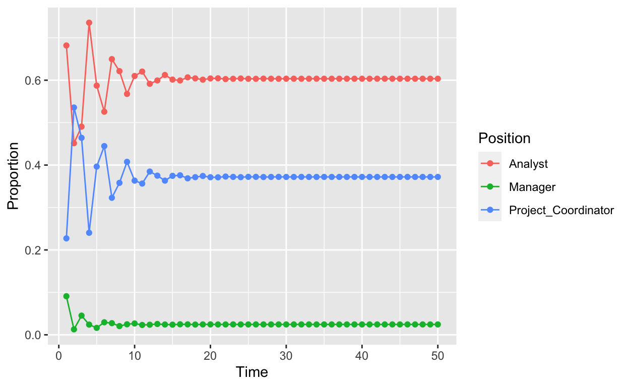
The Company Roles Over 50 Years:

df <- matrix(, nrow = 50, ncol = 3)

count <- 0

for(i in 1:50){
  count <- count + 1
  
  if(i == 1){
    
    df[count,] = initial
  
  }
  else{
    
    df[count,] = transition%^%i %*% initial
  }
  
}

If job-movement in a company aligned with our initial assumptions, we would expect the distribution of jobs to follow this pattern across time:

Some data tidying first…

df <- data.frame(df)
names(df) <- c("Analyst", "Project_Coordinator", "Manager")
df$Time <- rep(1:nrow(df))

data_f <- df %>%
  gather(Analyst, Project_Coordinator, Manager, key = "Position", value = "Num_People")

total_value <- data_f %>%
  group_by(Time) %>%
  summarise(
    total = sum(Num_People)
  )

data_f <- left_join(data_f, total_value)


data_f <- data_f %>%
  mutate(Proportion = Num_People / total)

The proportion of people in each position:

library(ggthemes)

ggplot(data_f, aes(x = Time, y = Proportion, color = Position)) + 
  geom_point() + 
  geom_line()

The amount of people in the company overall:

ggplot(data_f, aes(x = Time, y = Num_People, color = Position)) + 
  geom_point() + 
  geom_line()

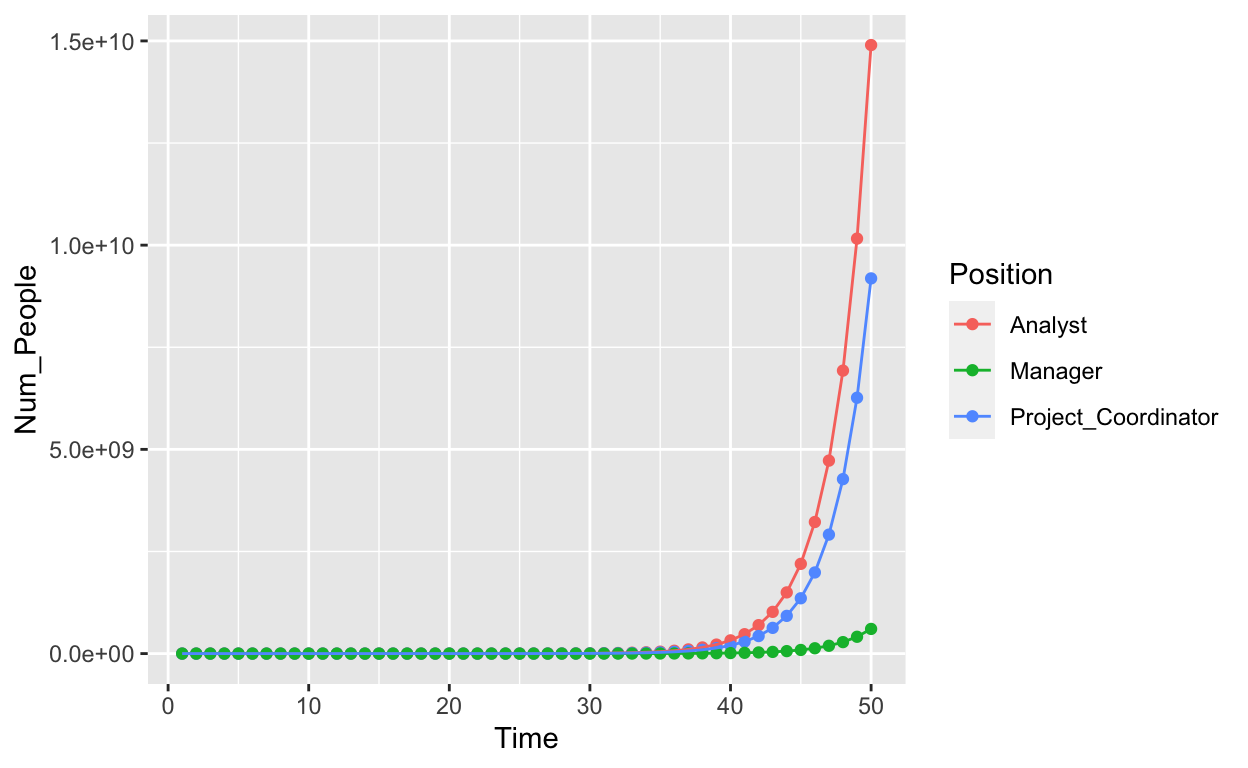
As you can tell, this is unrealistic =)

Bo\(^2\)m =)