A fun simulation by McClelland and Judd (1993) in Psychological Bulletin that demonstrates why detecting interactions outside the lab (i.e., in field studies) is difficult. In experiments, scores on the independent variables are located at the extremes of their respective distributions because we manipulate conditions. The distribution of scores across all of the independent variables in field studies, conversely, is typically assumed to be normal. By creating “extreme groups” in experiments, therefore, it becomes easier to detect interactions.
Imagine running an experiment where we randomly assign participants to one of two groups on an independent variable, goal difficulty. In one group the goal is challening, in the other group the goal is easy to accomplish. We are then interested in which group performs better on a task. After randomly assigning to groups, the distribution of scores on “goal difficulty” would be as follows:
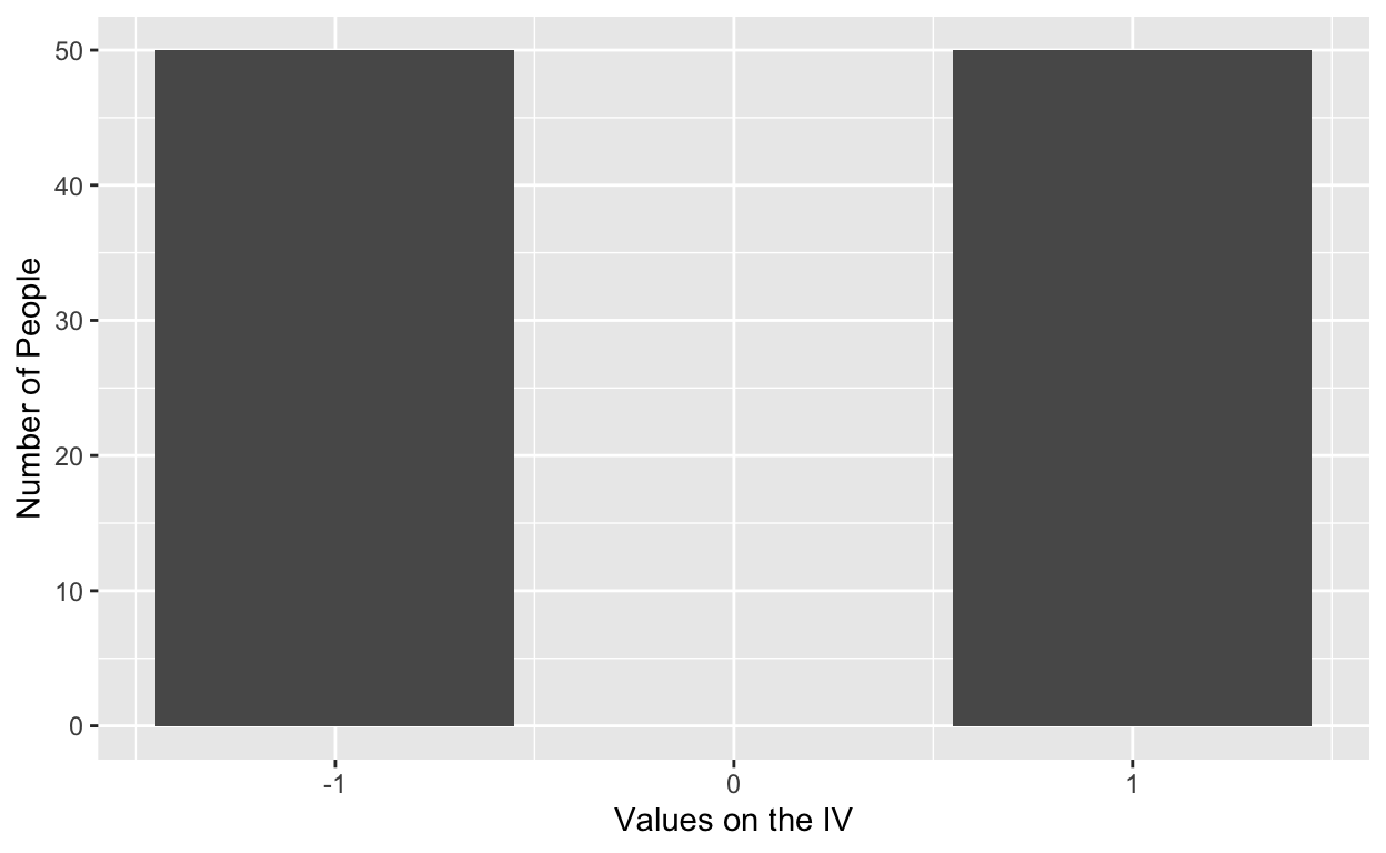
where 50 people are assigned to each condition. In this case, the distribution of scores is aligned at the extremes (i.e., -1, or the hard goal, and 1, or the easy goal) because we manipulated that variable. In field studies, where we cannot manipulate goal difficulty, the distribution of scores would be as follows:
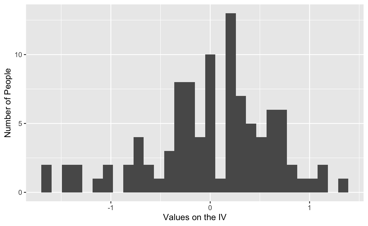
where scores about the independent variable (goal difficulty) are dispersed because we did not manipulate. The same distributional differences occur across other independent variables that we include in our design, and they are the reason behind fewer interaction detections in field studies.
The cool part is that this happens even when the data generating mechanisms are exactly the same. The mechanism that causes \(y\), in both the experiments and field studies in this simulation, will be:
\[\begin{equation} y_{i} = b_0{i} + b_1{x_i} + b_2{z_i} + b_3{zx_i} + e_{i} \end{equation}\]
where \(y_{i}\) is the value of the outcome (i.e., performance) for the \(i^\text{th}\) person, \(x_i\) is the value of one independent variable for the \(i^\text{th}\) person (i.e., goal difficulty), \(z_i\) is the value of another independent variable for the \(i^\text{th}\) person (e.g., whatever variable you please), \(zx_i\) represents the combination of values on \(x\) and \(z\) for the \(i^\text{th}\) person (i.e., the interaction term), \(e_i\) is a normally distributed error term for the \(i^\text{th}\) person, and \(b_0\), \(b_1\), and \(b_2\) represent the regression intercept and coefficients relating the predictors to the outcome.
Again, the data generating equation, the thing that causes \(y\), is the same for both field studies and experiments. We are going to find differences, however, simply because the distribution on the independent variables are different.
The values for \(b_0\), \(b_1\), and \(b_2\) will be, respectively, 0, 0.20, 0.10, and 1.0 (see McClelland & Judd, 1993). In other words, our interaction coefficient is gigantic.
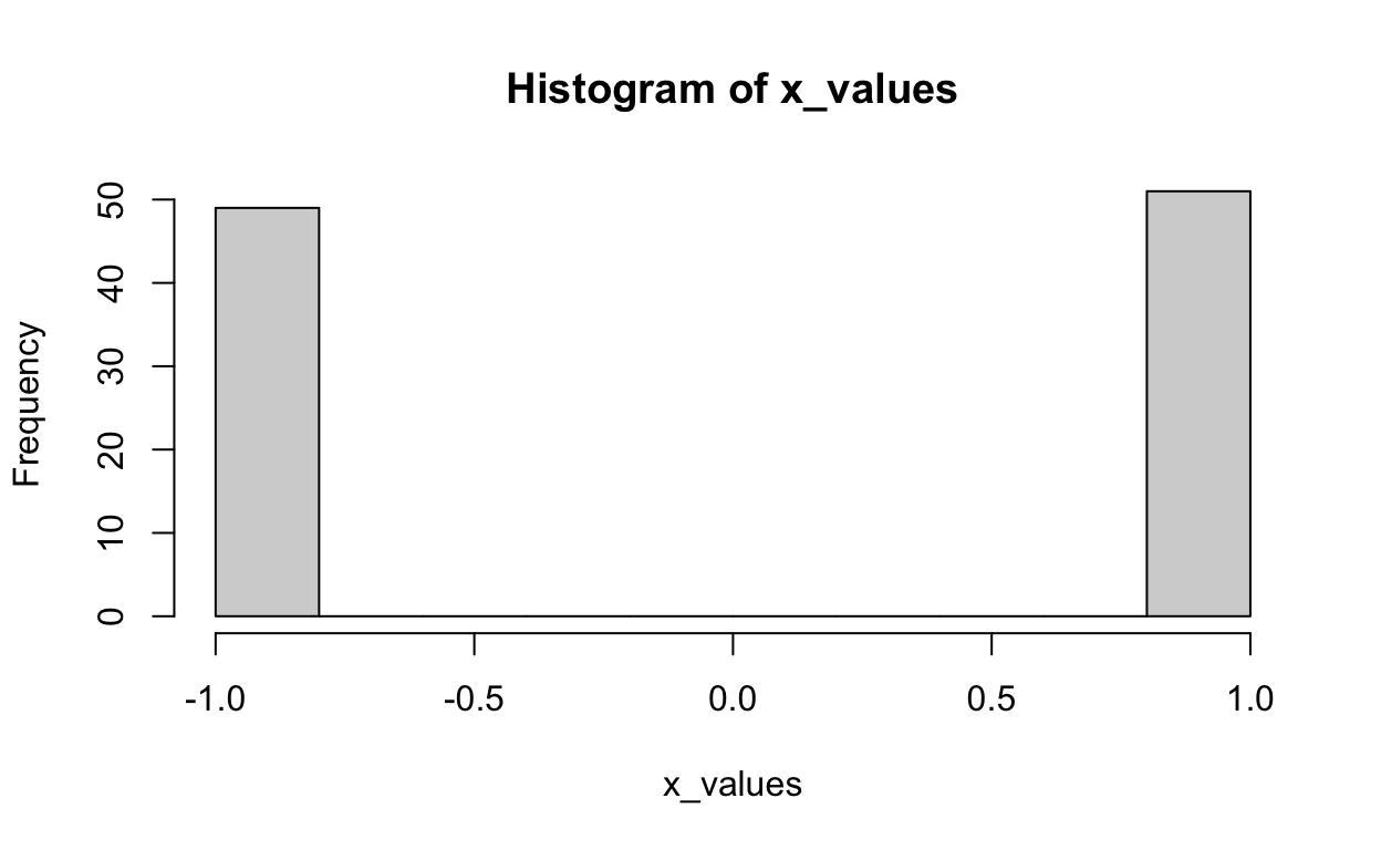
Each simulation will use the equation just presented to generate data across 100 individuals in the field and 100 individuals in the lab. The only difference between the two groups will be their initial distribution on \(x\) and \(z\). For the lab group, their scores will be randomly assigned to -1 or 1, and in the field group scores will be randomly dispersed (normally) between -1 and 1. After generating the data I then estimate the coefficients using multiple regression and save the significance value in a vector. The process then interates 1000 times.
The Experiment Data
The distribution of X:
The distribution of Z:

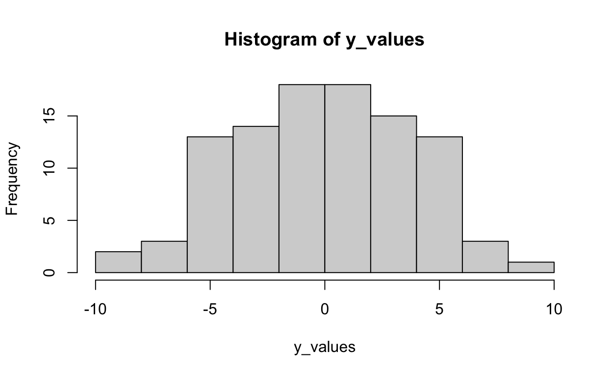
The distribution of Y after using the equation above to generate scores on Y:
y_values <- b_0 + 0.20*x_values + 0.10*z_values +
            1.00*x_values*z_values + rnorm(100,0,4)

hist(y_values)
Now estimate the parameters using regression:
exp_data <- data.frame("X" = c(x_values),
                       "Z" = c(z_values),
                       "Y" = c(y_values))

exp_model <- lm(Y ~ X + Z + X:Z, data = exp_data)
summary(exp_model)
Call:
lm(formula = Y ~ X + Z + X:Z, data = exp_data)

Residuals:
    Min      1Q  Median      3Q     Max
-9.5221 -2.5763  0.3173  2.9709  8.2962

Coefficients:
            Estimate Std. Error t value Pr(>|t|)
(Intercept) -0.14473    0.38409  -0.377  0.70715
X           -0.06575    0.38409  -0.171  0.86444
Z           -0.24140    0.38409  -0.628  0.53117
X:Z          1.06693    0.38409   2.778  0.00658 **
---
Signif. codes:  0 '***' 0.001 '**' 0.01 '*' 0.05 '.' 0.1 ' ' 1

Residual standard error: 3.777 on 96 degrees of freedom
Multiple R-squared:  0.08142,   Adjusted R-squared:  0.05272
F-statistic: 2.836 on 3 and 96 DF,  p-value: 0.04215
The Field Study Data
The distribution of X:
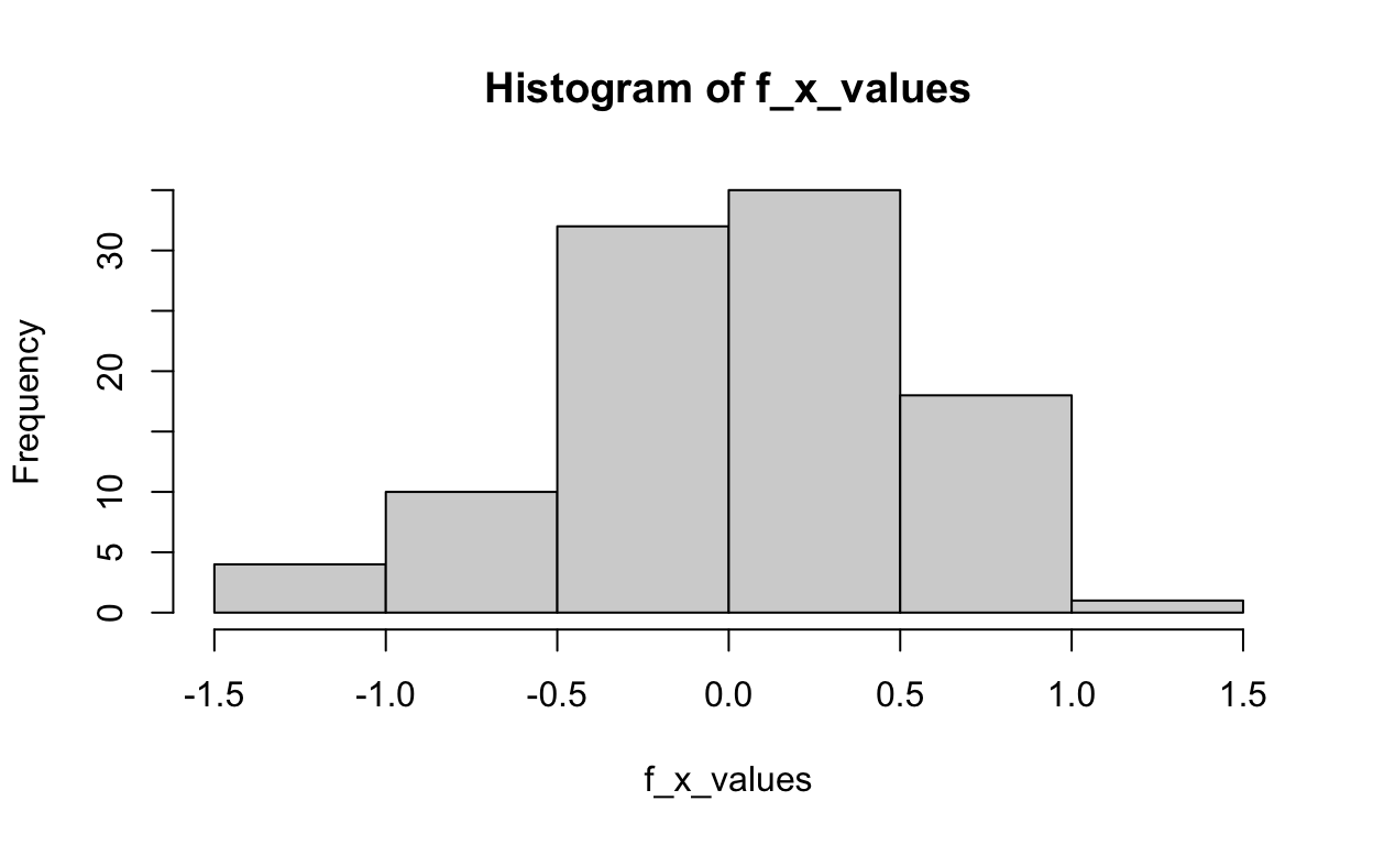
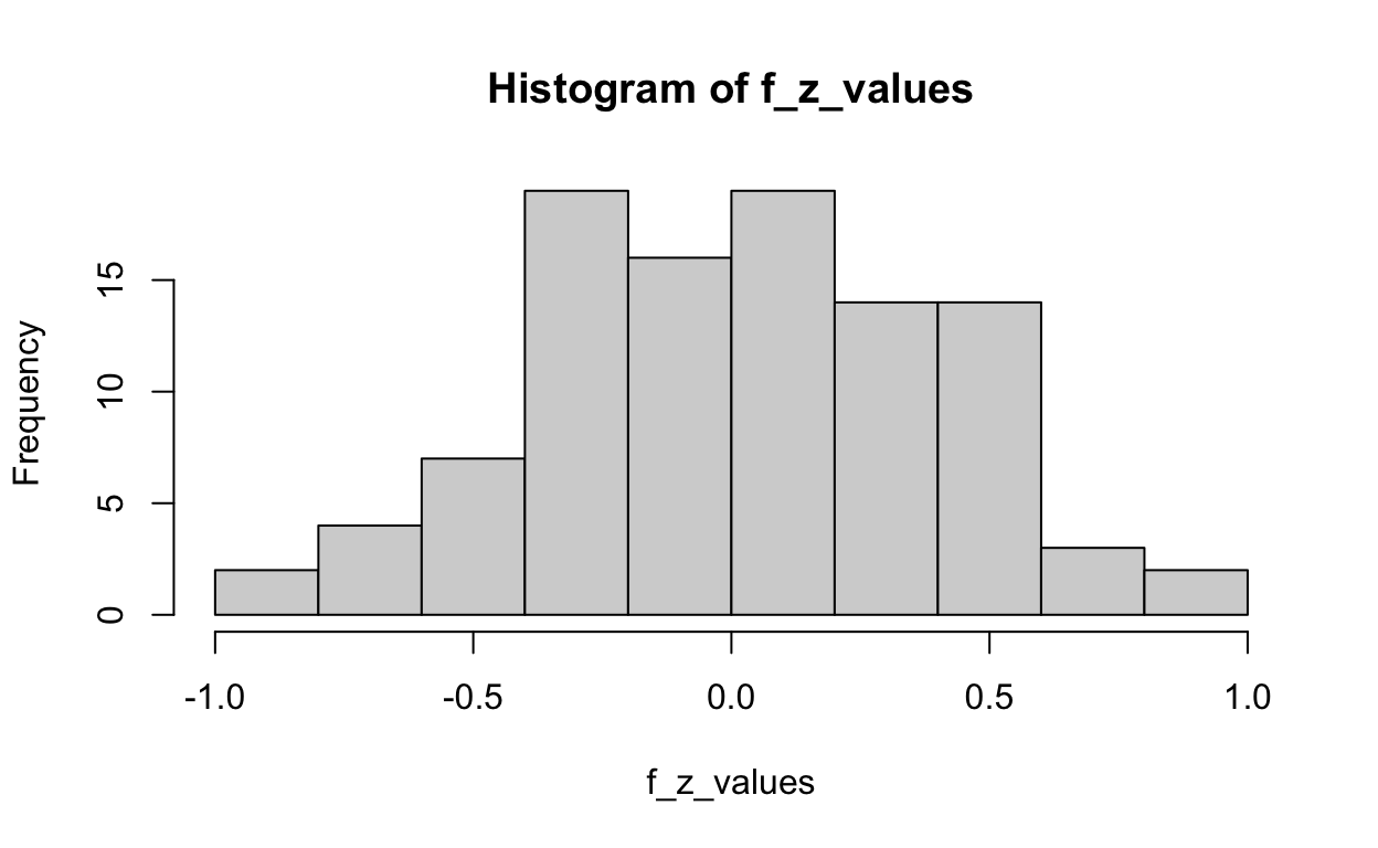
The distribution of Z:
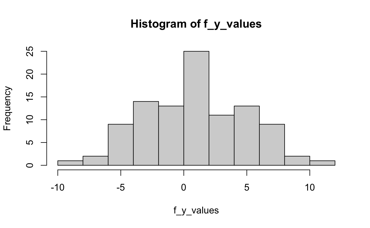
The distribution of Y after using the equation above to generate scores on Y:
f_y_values <- b_0 + 0.20*f_x_values + 0.10*f_z_values +
              1.00*f_x_values*f_z_values + rnorm(100,0,4)

hist(f_y_values)
Now estimate the parameters using regression:
field_data <- data.frame("FX" = c(f_x_values),
                           "FZ" = c(f_z_values),
                           "FY" = c(f_y_values))

field_model <- lm(FY ~ FX + FZ + FX:FZ, data = field_data)
summary(field_model)
Call:
lm(formula = FY ~ FX + FZ + FX:FZ, data = field_data)

Residuals:
   Min     1Q Median     3Q    Max
-9.394 -2.967  0.134  2.868 11.158

Coefficients:
            Estimate Std. Error t value Pr(>|t|)
(Intercept)  0.97308    0.40804   2.385   0.0191 *
FX          -0.04196    0.82524  -0.051   0.9596
FZ          -1.36550    1.04609  -1.305   0.1949
FX:FZ        1.34535    2.19279   0.614   0.5410
---
Signif. codes:  0 '***' 0.001 '**' 0.01 '*' 0.05 '.' 0.1 ' ' 1

Residual standard error: 4.057 on 96 degrees of freedom
Multiple R-squared:  0.02166,   Adjusted R-squared:  -0.008912
F-statistic: 0.7085 on 3 and 96 DF,  p-value: 0.5492
Putting Everything Into Monte Carlo
Replicate the process above 1000 times and save the p-value each time
sims <- 1000
exp_results <- numeric(1000)
field_results <- numeric(1000)


X_coefficient <- 0.20
Z_coefficient <- 0.10

XZ_coefficient <- 1.00
Mu <- 0

xy_data <- c(-1,1)

library(MASS)

for(i in 1:sims){

  # Experiment Data

  # X
  x_values <- sample(xy_data, 100, replace = T)

  # Z
  z_values <- sample(xy_data, 100, replace = T)

  # Y
  y_values <- Mu + X_coefficient * x_values + Z_coefficient * z_values +
              XZ_coefficient * x_values * z_values + rnorm(100,0,4)

  exp_data <- data.frame("X" = c(x_values),
                         "Z" = c(z_values),
                         "Y" = c(y_values))


  # Field Data

  # X
  f_x_values <- rnorm(100, 0, 0.5)

  # Z
  f_z_values <- rnorm(100, 0, 0.5)

  # Y
  f_y_values <- Mu + X_coefficient * f_x_values + Z_coefficient * f_z_values +
                XZ_coefficient * f_x_values * f_z_values + rnorm(100,0,4)


  field_data <- data.frame("FX" = c(f_x_values),
                           "FZ" = c(f_z_values),
                           "FY" = c(f_y_values))


  # Modeling


  exp_model <- lm(Y ~ X + Z + X:Z, data = exp_data)
  exp_results[i] <- summary(exp_model)$coefficients[4,4]

  field_model <- lm(FY ~ FX + FZ + FX:FZ, data = field_data)
  field_results[i] <- summary(field_model)$coefficients[4,4]

}
The Results
What proportion of experiments find significant interaction effects?
sum(exp_results < 0.05) / 1000
[1] 0.669What proportion of field studies find significant interaction effects?
sum(field_results < 0.05) / 1000
[1] 0.086Bo\(^2\)m =)