I like to think of Monte Carlo as a counting method. If a condition is satisfied we make a note (e.g., 1), and if the condition is not satisfied we make a different note (e.g., 0). We then iterate and evaluate the pattern of 1’s and 0’s to learn about our process. Art can be described in a similar way: if a condition is satisfied we use a color, and if a condition is not satisfied we use a different color. After many iterations, we have an image.
Here is a simulation that “draws” a process, inspired by Caleb Madrigal (link here).
The Data Generating Process
Some Initial Values
x <- seq(0, 10, length.out = 1000)
Using the DGP to generate values of Y
y <- f(x)

plot(x, y)
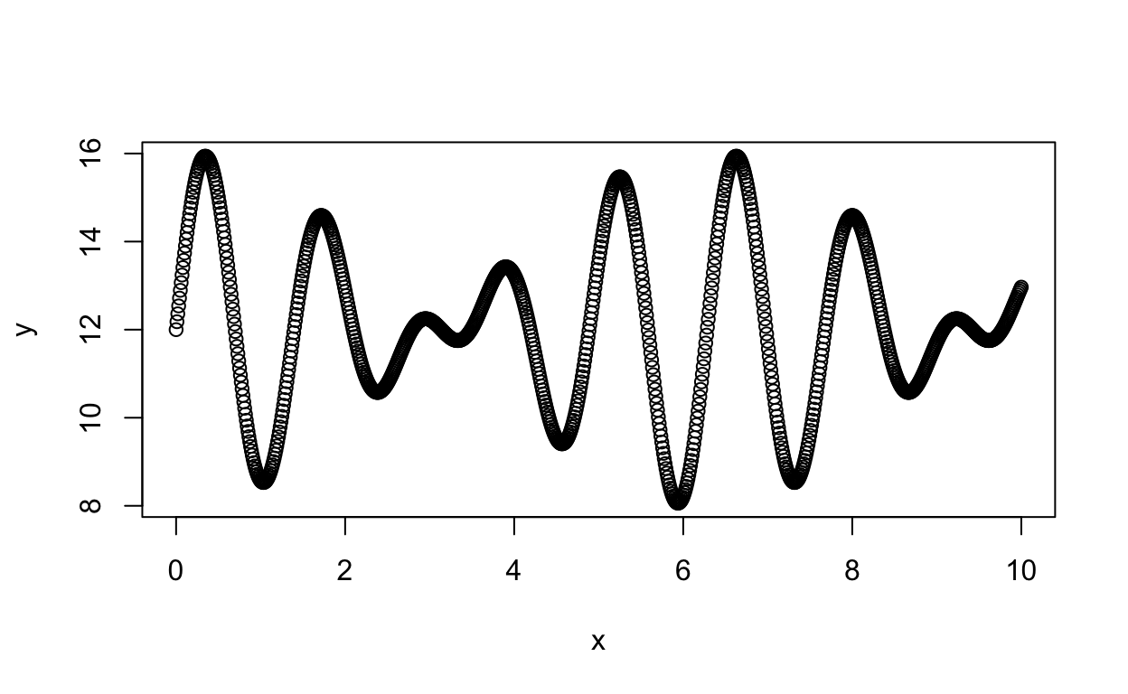
This is the process we want to “draw”
Now for the Monte Carlo
We are going to evaluate 10,000 points within our process space (10 x 16).
num_points <- 10000
rect_width <- 10
rect_height <- 16

points <- matrix(, ncol = 2, nrow = num_points)
Column 1 of our points matrix represents the width of our process space while column 2 represents its height. First we fill the matrix with random values within our process space:
Now we iterate across all of those points and evaluate them with respect to our process. Think of the “width” as X values and the “height” as Y values. Given a value of X, is our random value of Y less than it would be if we created a Y value by using our function (f(x))? If so, mark it in the “points_under” vector. If not, mark it in the “points_over” vector.
points_under = matrix(, ncol = 2, nrow = num_points)
points_above = matrix(, ncol = 2, nrow = num_points)

for(i in 1:num_points){
  if(points[i,2] < f(points[i,1])){
    points_under[i,1] <- points[i,1]
    points_under[i,2] <- points[i,2]
  }
  else{
    points_above[i,1] <- points[i,1]
    points_above[i,2] <- points[i,2]
  }
}
Put the results into new vectors without NA’s. Some NA’s come up because our data generating process is crazy.
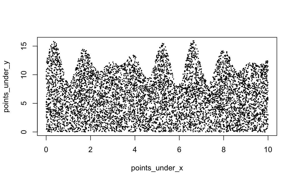
Now we have an image…
plot(points_under_y ~ points_under_x, pch = 20, cex = 0.3)
Bo\(^2\)m =)