Here’s how to approximate a differential equation using discrete simulations in R. Differential equations will be presented in the form
\[\begin{equation} \frac{dx}{dt} \end{equation}\]
where \(dx\) is the change in whatever stock \(x\) represents and \(dt\) is the length of the time step. Any differential equation can be rearranged as
\[\begin{equation} dx = f() * dt. \end{equation}\]
where some function is multiplied by the time step \(dt\). In R, you could make this time step 0.000001, which is close enough to continuous that it often approximates functions well. Once you calculate \(dx\), or the change in \(x\) over a small time step (i.e., 0.000001), then you can add this change to the current value of \(x\):
\[\begin{equation} x_{new} = x + dx \end{equation}\]
Rinse and repeat. Here is an example using the famous Lotka-Volterra Equations. Predator-Prey dynamics can be modeled with:
\[\begin{equation} \frac{dx}{dt} = Ax - Bxy \end{equation}\]
\[\begin{equation} \frac{dy}{dt} = Cxy - Dy \end{equation}\]
where
- \(x\) is the number of prey
- \(y\) is the number of predators
- \(A\) is the birth rate of prey
- \(B\) is the contact rate between predators and prey
- \(C\) can either be equivalent to \(B\), or it can be thought of as the predator birth rate due to the presence of prey
- \(D\) is the death rate of predators in the absence of prey
- \(dx\) is the change in number of prey
- \(dy\) is the change in the number of predators
- \(dt\) is the time step (not number of time points).
We can numerically approximate these equations by multiplying each equation by \(dt\) and then simulating with a small time step (e.g., 0.0001).
A discrete time version would be:
dx <- (Ax - Bxy) * small_step
dy <- (Cxy - Dy) * small_step

x_new <- x + dx
y_new <- y + dy

repeat many times...
Let’s run it.
step <- 0.1
time <- seq(from = step, to = 100, by = step)
x <- numeric(length(time))
y <- numeric(length(time))
x[1] <- 3
y[1] <- 5
A <- 1
B <- 0.2
C <- 0.04
D <- 0.5

count <- 0
for(i in time){
  count <- count + 1


  dx <- (A*x[count] - B*x[count]*y[count]) * step
  dy <- (C*x[count]*y[count] - D*y[count]) * step

  x_new <- x[count] + dx
  y_new <- y[count] + dy

  x[count + 1] <- x_new
  y[count + 1] <- y_new


}
library(tidyverse)
library(ggplot2)
library(hrbrthemes)

df <- data.frame(
  'time' = c(time, time),
  'val' = c(x[1:length(time)], y[1:length(time)]),
  'var' = c(rep("Prey", length(time)),
            rep("Predator", length(time)))
)


ggplot(df, aes(x = time, y = val, color = var)) +
  geom_line() +
  theme_ipsum()
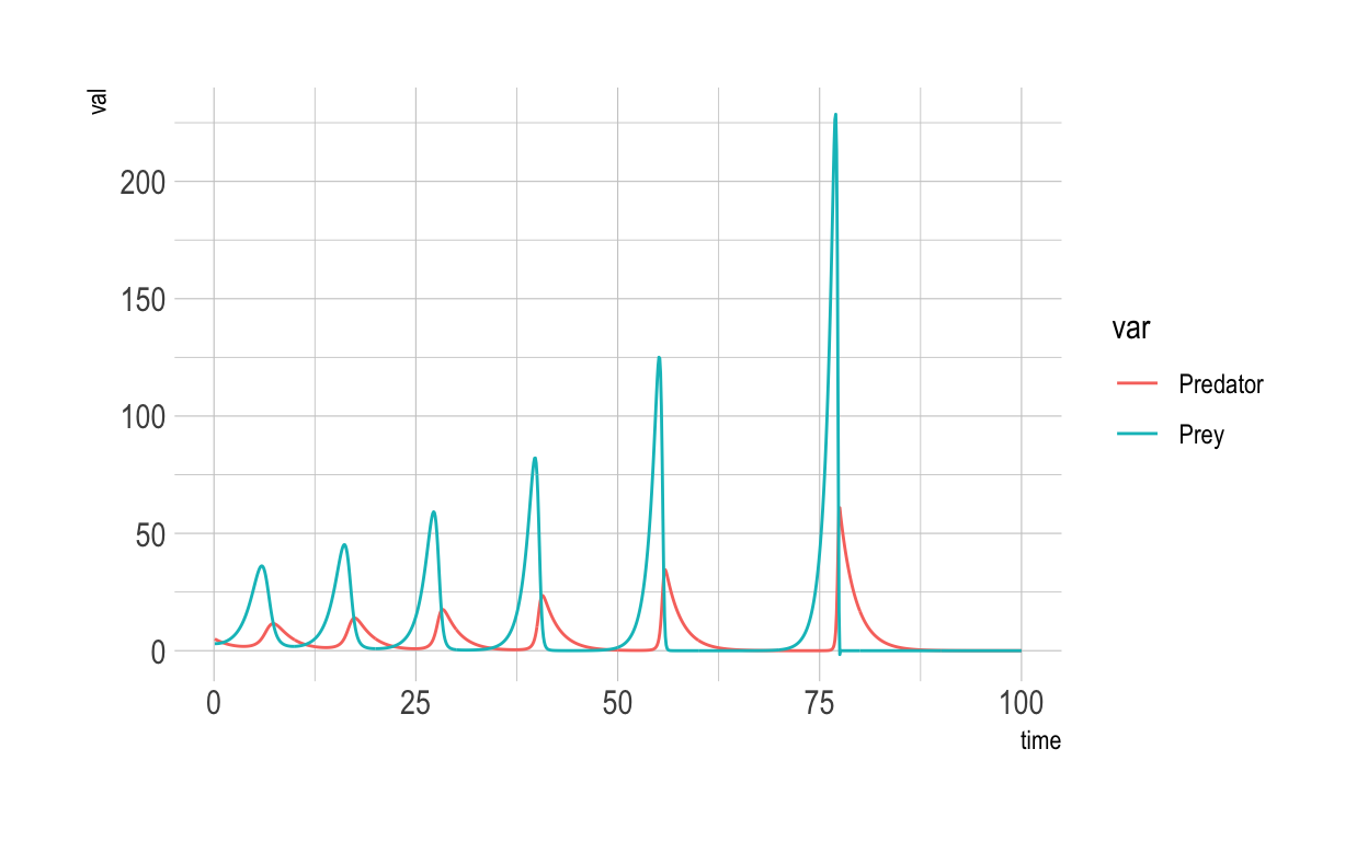
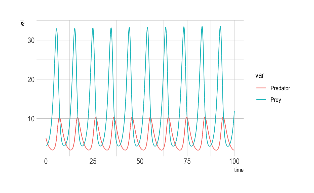
Cool. The ever-growing size of the spikes is an artifact of approximation. Let’s use an even smaller step:
step <- 0.001
Here is the output:
In these simulations, I used what I call a “push forward” approach (i.e., generate x at t + 1 from x current). Sometimes, I prefer to use a “look backward” approach (i.e., generate x from x at t - 1). Here is the second approach:
step <- 0.001
time <- 1000
x <- numeric(length(time))
y <- numeric(length(time))
x[1] <- 3
y[1] <- 5
A <- 1
B <- 0.2
C <- 0.04
D <- 0.5

for(i in 2:time){


  dx <- (A*x[i - 1] - B*x[i - 1]*y[i - 1]) * step
  dy <- (C*x[i - 1]*y[i - 1] - D*y[i - 1]) * step

  x_new <- x[i - 1] + dx
  y_new <- y[i - 1] + dy

  x[i] <- x_new
  y[i] <- y_new


}
Bo\(^2\)m =)