The Schelling model that I created in my last script used matrix operations. It required me to think in terms of patches housed in a matrix. Consider the following 3x3 grid.
     [,1] [,2] [,3]
[1,]    1    1    0
[2,]    0    2    2
[3,]    1    0    0
Each cell can be thought of as a patch. When a given patch is 0, it is unoccupied. When a given patch is 1 or 2, it is occupied by a hockey or soccer player, respectively. When I implement a Schelling model using a matrix, it puts me in a certain frame of mind. I have to consider patches as locations specified by rows and columns. At row 1 column 2, for example, sits patch XXX that is either occupied or unoccupied.
Another way to implement the Schelling model is to use long data. The same information conveyed in the 3x3 matrix is shown in long form below.
  xcoord ycoord type
1      1      1    1
2      2      1    0
3      3      1    1
4      1      2    1
5      2      2    2
6      3      2    0
7      1      3    0
8      2      3    2
9      3      3    0
Coordinates are now viewed as information that can be stored in respective columns. The type column represents whether the patch is unoccupied (0), houses a hockey player (1), or houses a soccer player (2). The goal of this post is to re-create the Schelling model using long data.
I’m going to present the code in two sections. The first demonstrates the behavior of 1 agent within a single time point. The second reveals the full model: it iterates over 50 time points using all agents.
Basic Idea
The model uses two data frames to store (the most important) information. One holds the coordinates of the living location of each agent. Susan, for example, lives at xcoord = 3 & ycoord = 10, whereas Johnny lives at xcoord = 2 & ycoord = 15. The other specifies the object located at each patch on the grid (0 = unoccupied, 1 = hockey player, 2 = soccer player), and this second data frame will be used for plotting.
To reiterate, one data frame stores agent coordinates:
library(kableExtra)

head(agent_df) %>%
  kable() %>%
  kable_styling()
| xcoord | ycoord | type | agent |
|---|---|---|---|
| 1 | 1 | 1 | 1 |
| 2 | 1 | 1 | 2 |
| 5 | 1 | 1 | 3 |
| 6 | 1 | 1 | 4 |
| 7 | 1 | 2 | 5 |
| 8 | 1 | 1 | 6 |
and the other, which will be used for plotting, stores patch information.
head(patch_df) %>%
  kable() %>%
  kable_styling()
| xcoord | ycoord | type |
|---|---|---|
| 1 | 1 | 1 |
| 2 | 1 | 1 |
| 3 | 1 | 0 |
| 4 | 1 | 0 |
| 5 | 1 | 1 |
| 6 | 1 | 1 |
The pseudocode for the model is as follows.
"
for each period

    for each agent i

        identify i's 8 surrounding neighbors
        count the number of similar and dissimilar neighbors
        -- e.g., if i is a hockey player and is surrounded by soccer players...
        -- then he has mostly dissimilar neighbors

        if agent i has more dissimilar neighbors than he desires, then label him as unhappy
        if agent i has more similar neighbors than he desires, then label him as happy

        repeat for all agents

    for each unhappy agent j

        randomly select a new patch to possibly move to
        if the patch is unoccupied, move there

        repeat for all unhappy agents


    plot the grid of patches for this period
    save the plot

end
"
Of course, the model is much more complex in syntax. But the basic idea is straightforward: people move if they have many dissimilar neighbors, and they stay if they have similar neighbors. Moreover, new patches, which are selected when agents want to move, are pulled randomly.
Let’s pretend we are at the first period and are beginning to iterate across agents. The code works as follows.
Starting with agent 1, identify her coordinates and type (type meaning hockey or soccer player).
    agent_coords <- agent_df %>%
      filter(agent == 1) %>%
      select(xcoord, ycoord)

    agent_type <- agent_df %>%
      filter(agent == 1) %>%
      select(type) %>%
      pull()


glimpse(agent_coords)
Rows: 1
Columns: 2
$ xcoord <int> 1
$ ycoord <int> 1glimpse(agent_type)
num 1Using agent i’s coordinates, identify her 8 surrounding neighbors.
neigh <- get_neigh(agent_coords)
The function get_neigh is prespecified (I will show you the syntax below). It’s too complicated to pick apart now. Just know that it returns the coordinates of her 8 surrounding neighbors.
I’m about to start counting similar neighbors, so I need to initialize a few counters.
total_neighs <- 0
similar_neighs <- 0
Count similar neighbors. Go through each row in the neigh matrix to find a given neighbor’s coordinates. Use those coordinates to pull all information about neighbor n from the agent data frame. Then, increment similar_neighs by 1 if neighbor n is the same type as agent i. Increment total_neighs if the patch isn’t empty.
Stated simply, if agent i is a hockey player then count the number of other hockey players. Also count the number of non-empty patches.
    for(n in 1:nrow(neigh)){

      # save neighbor
      neigh_agent <- patch_df %>%
        filter(xcoord == neigh$xcoord[n],
               ycoord == neigh$ycoord[n])

      # increment similar neighbors by 1 if agent is same as neighbor
      # increment total neighbors by 1 if patch isn't empty
      if(agent_type == neigh_agent$type){similar_neighs <- similar_neighs + 1}
      if(neigh_agent$type != 0){total_neighs <- total_neighs + 1}

    }
Now my counters have values.
Total Neighbors = 4
Similar Neighbors = 3
Calculate a similarity ratio. Take the number of similar neighbors and divide it by the total number of neighbors (i.e., non-empty patches).
sim_ratio <- similar_neighs / total_neighs
I won’t show the code here, but all of the information calculated so far then gets stored in a master “results” data frame.
So far, we have identified agent i’s neighbors and calculated her similarity ratio. We now need to determine whether she wants to move. If she does, we then need to find a new place for her to move to.
Schelling’s original model used inequalities to generate agent happiness (or satisfaction). When one’s similarity ratio is greater than some innate preference for similar others (say, 0.6), then the agent is happy and stays put. When one’s similarity ratio is lower than 0.6, the agent is unhappy and moves. Here is that idea embodied in code.
empty <- is.nan(sim_ratio)
happy <- NULL

if(empty == TRUE){happy <- TRUE} # if the agent has no neighbors, he is happy
if(empty == FALSE && sim_ratio > 0.6){happy <- TRUE}
if(empty == FALSE && sim_ratio < 0.6){happy <- FALSE}
if(empty == FALSE && sim_ratio == 0.6){happy <- FALSE}
The inequalities are located in the if statements. What makes the syntax a bit tricky is that I also included an empty object. I did that because not all agents have neighbors. It is possible for an agent to be surrounded by all empty patches. When this (unlikely) case happens, then total_neighs is equal to 0, and we all know that dividing by 0 doesn’t work. So, the code above asks whether sim_ratio has an actual value, and it only moves forward if so. Said differently, empty would equal TRUE when agent i has no neighbors. If the agent is happy, the code moves forward. If the agent is unhappy, she gets stored (not shown).
The steps above then repeat for every agent. Once it iterates over all agents, storing the unhappy agents when they arise, it finds new patches for the unhappy agents. First, randomly select new coordinates.
Is the patch located at those coordinates occupied?
If the patch is unoccupied, then we can work with our unhappy agent. If the patch is occupied, we need to continue to sample patches until we find one that is unoccupied.
Once selected, we change the new patch to occupied within the patch_df, change the old patch to unoccupied within the patch_df, and update the agent data frame with unhappy agent i’s new coordinates. The code to do so is something like the following.
# change new patch to unhappy agent i's type
patch_df[patch_df$xcoord == new_x & patch_df$ycoord == new_y, "type"] <- current_unhappy$type[1]
# go to the old patch where unhappy agent i used to live and change it to 0
patch_df[patch_df$xcoord == current_unhappy$xcoord[1] & patch_df$ycoord == current_unhappy$ycoord[1], "type"] <- 0
# update the agent_df to reflect unhappy agent i's new coordinates
agent_df[agent_df$agent == current_unhappy$agent[1], "xcoord"] <- new_x
agent_df[agent_df$agent == current_unhappy$agent[1], "ycoord"] <- new_y
Full Model
Here is the full model.
library(tidyverse)
library(reshape2)
library(ggplot2)
# initial grid
#
#
#
#
#
#
dims <- 51*51
empty_patches <- 781
peeps <- c(rep(1, (dims-empty_patches) / 2),
rep(2, (dims-empty_patches) / 2),
rep(0, empty_patches))
num_agents <- dims - empty_patches
mat <- matrix(sample(peeps, dims, replace = F), 51, 51, byrow = T)
patch_df <- melt(mat) %>%
mutate(xcoord = Var1,
ycoord = Var2,
type = value) %>%
select(xcoord,
ycoord,
type)
agent_df <- patch_df %>%
filter(type %in% c(1,2)) %>%
mutate(agent = 1:num_agents)
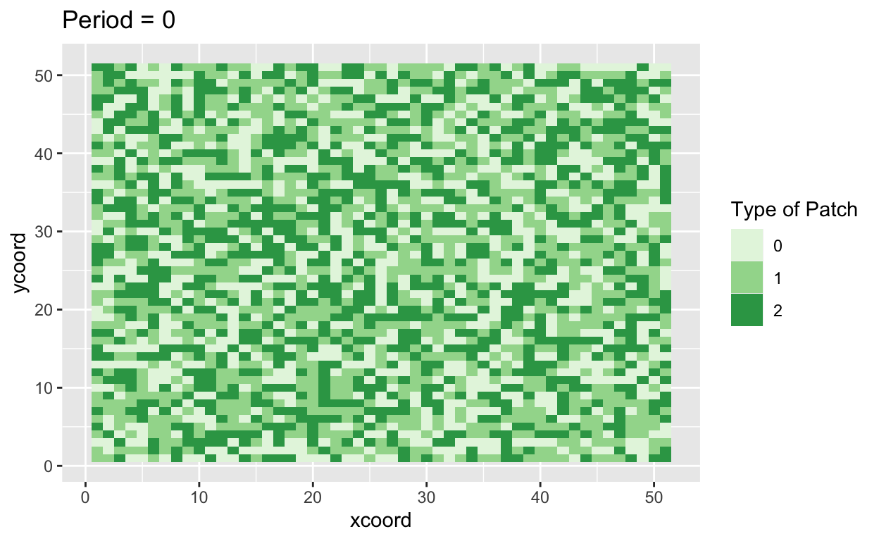
plotfirst <- patch_df
alike_preference <- 0.6
# get neighbors function
#
#
#
#
#
#
#
#
get_neigh <- function(xy){
# starting from right and going clockwise, I want neighbors a,b,c,d,e,f,g,h
ax <- xy[1 , "xcoord"] + 1
ay <- xy[1, "ycoord"]
# xcoord, ycoord
a <- c(ax, ay)
bx <- xy[1 , "xcoord"] + 1
by <- xy[1, "ycoord"] - 1
# xcoord, ycoord
b <- c(bx, by)
cx <- xy[1 , "xcoord"]
cy <- xy[1, "ycoord"] - 1
# xcoord, ycoord
c <- c(cx, cy)
dx <- xy[1 , "xcoord"] - 1
dy <- xy[1, "ycoord"] - 1
# xcoord, ycoord
d <- c(dx, dy)
ex <- xy[1 , "xcoord"] - 1
ey <- xy[1, "ycoord"]
# xcoord, ycoord
e <- c(ex, ey)
fx <- xy[1 , "xcoord"] - 1
fy <- xy[1, "ycoord"] + 1
# xcoord, ycoord
f <- c(fx, fy)
gx <- xy[1 , "xcoord"]
gy <- xy[1, "ycoord"] + 1
# xcoord, ycoord
g <- c(gx, gy)
hx <- xy[1 , "xcoord"] + 1
hy <- xy[1, "ycoord"] + 1
# xcoord, ycoord
h <- c(hx, hy)
dff <- data.frame(
'xcoord' = c(a[1], b[1], c[1], d[1], e[1], f[1], g[1], h[1]),
'ycoord' = c(a[2], b[2], c[2], d[2], e[2], f[2], g[2], h[2])
)
dff <- dff %>%
mutate(xcoord = ifelse(xcoord == 0, 51, xcoord),
xcoord = ifelse(xcoord == 52, 1, xcoord),
ycoord = ifelse(ycoord == 0, 51, ycoord),
ycoord = ifelse(ycoord == 52, 1, ycoord))
return(dff)
}
# initialize stores
#
#
#
#
#
#
#
#
#
time <- 40
result_df <- data.frame(
"time" = numeric(time*num_agents),
"agent" = numeric(time*num_agents),
"simratio" = numeric(time*num_agents)
)
count <- 0
save_plots <- list()
# begin iterations over periods
#
#
#
#
#
#
#
for(i in 1:time){
unhappy_store <- list()
unhappy_counter <- 0
# for each agent
for(ag in 1:num_agents){
count <- count + 1
# save agent's coords
# save agent's type
agent_coords <- agent_df %>%
filter(agent == ag) %>%
select(xcoord, ycoord)
agent_type <- agent_df %>%
filter(agent == ag) %>%
select(type) %>%
pull()
# identify neighbors - save their coordinates
neigh <- get_neigh(agent_coords)
total_neighs <- 0
similar_neighs <- 0
# for each neighbor
for(n in 1:nrow(neigh)){
# save neighbor
neigh_agent <- patch_df %>%
filter(xcoord == neigh$xcoord[n],
ycoord == neigh$ycoord[n])
# increment similar neighbors by 1 if agent is same as neighbor
# increment total neighbors by 1 if patch isn't empty
if(agent_type == neigh_agent$type){similar_neighs <- similar_neighs + 1}
if(neigh_agent$type != 0){total_neighs <- total_neighs + 1}
}
# save his sim/total (time, agent, simratio)
sim_ratio <- similar_neighs / total_neighs
result_df[count, "time"] <- i
result_df[count, "agent"] <- ag
result_df[count, "simratio"] <- sim_ratio
# if the agent has empty patches around him (is.nan(sim_ratio) == T)
# or
# if sim/total > then alike_preferences,
# then the agent is happy
# otherwise, he is unhappy
empty <- is.nan(sim_ratio)
happy <- NULL
if(empty == TRUE){happy <- TRUE}
if(empty == FALSE && sim_ratio > alike_preference){happy <- TRUE}
if(empty == FALSE && sim_ratio < alike_preference){happy <- FALSE}
if(empty == FALSE && sim_ratio == alike_preference){happy <- FALSE}
# if the agent is unhappy, store him
if(happy == FALSE){
unhappy_counter <- unhappy_counter + 1
unhappy_store[[unhappy_counter]] <- ag
}
}
# after going through all agents, have the unhappy agents move
unhappy_agents <- unlist(unhappy_store)
for(q in 1:length(unhappy_agents)){
if(is.null(unhappy_agents) == TRUE){break}
# randomly select a new patch
  new_x <- sample(51, 1)
  new_y <- sample(51, 1)
# is the new patch occupied?
agent_type_at_new <- patch_df %>%
filter(xcoord == new_x,
ycoord == new_y) %>%
select(type) %>%
pull()
occupied <- FALSE
if(agent_type_at_new != 0){occupied <- TRUE}
  while(occupied == TRUE){

    new_x <- sample(51, 1)
    new_y <- sample(51, 1)
    agent_type_at_new <- patch_df %>%
      filter(xcoord == new_x,
             ycoord == new_y) %>%
      select(type) %>%
      pull()

    if(agent_type_at_new == 0){occupied <- FALSE}
  }
# unhappy agent
current_unhappy <- agent_df %>%
filter(agent == unhappy_agents[q])
# go to the new x and y position in the patch and place the agent type there
patch_df[patch_df$xcoord == new_x & patch_df$ycoord == new_y, "type"] <- current_unhappy$type[1]
# go to the old x and y position in the patch and change it to 0
patch_df[patch_df$xcoord == current_unhappy$xcoord[1] & patch_df$ycoord == current_unhappy$ycoord[1], "type"] <- 0
# change the agent_df to reflect the agent's new position
agent_df[agent_df$agent == current_unhappy$agent[1], "xcoord"] <- new_x
agent_df[agent_df$agent == current_unhappy$agent[1], "ycoord"] <- new_y
}
# create plot
# save and store plot
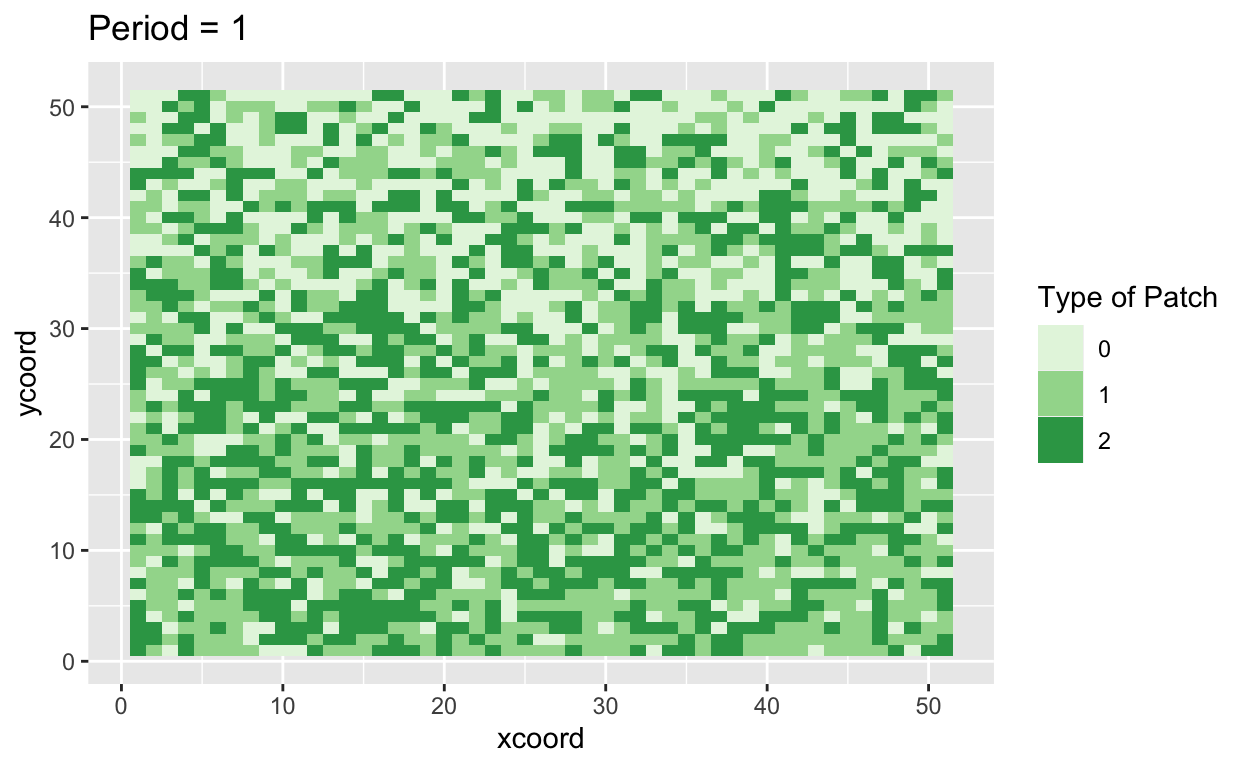
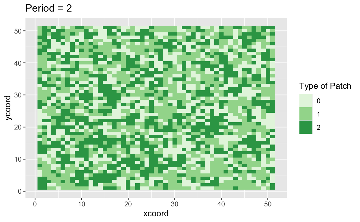
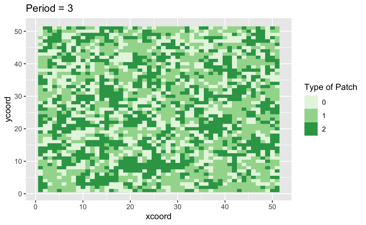
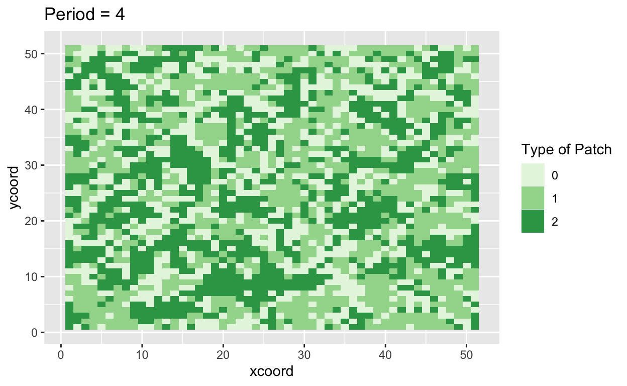
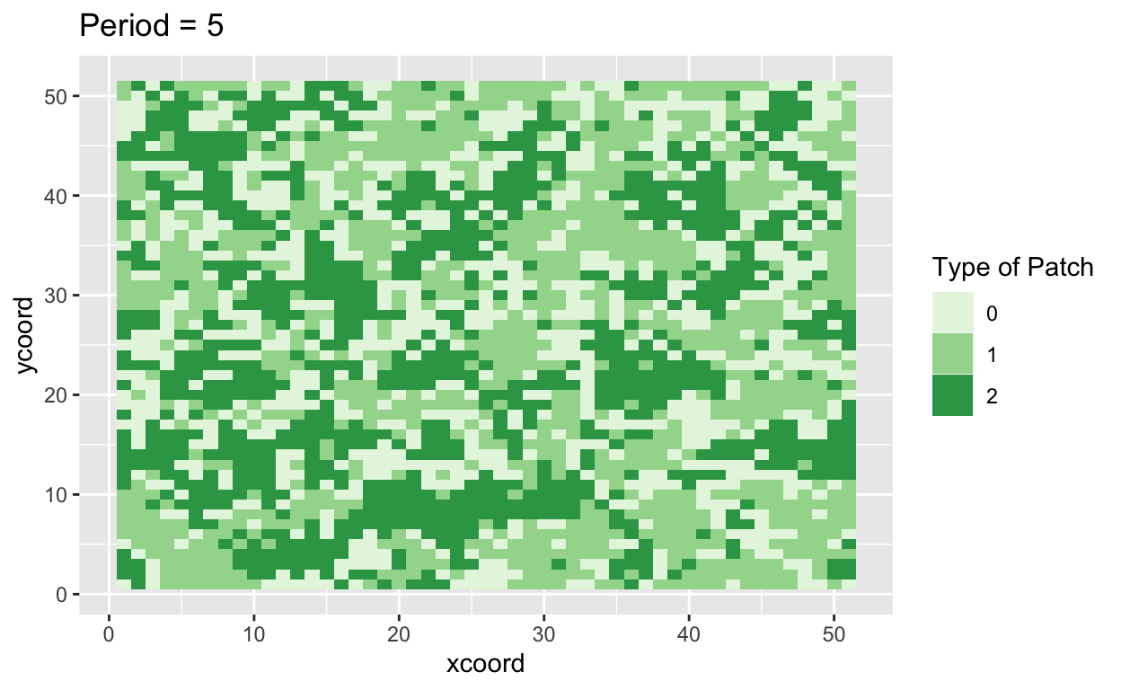
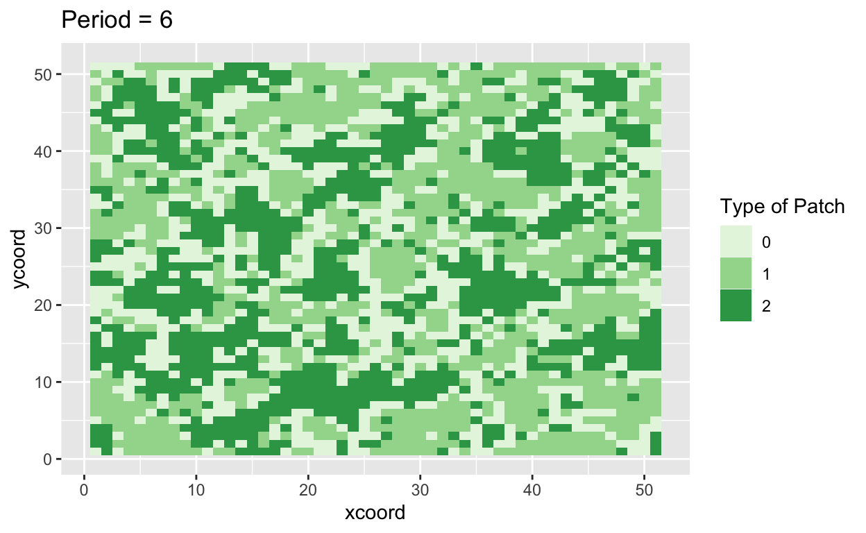
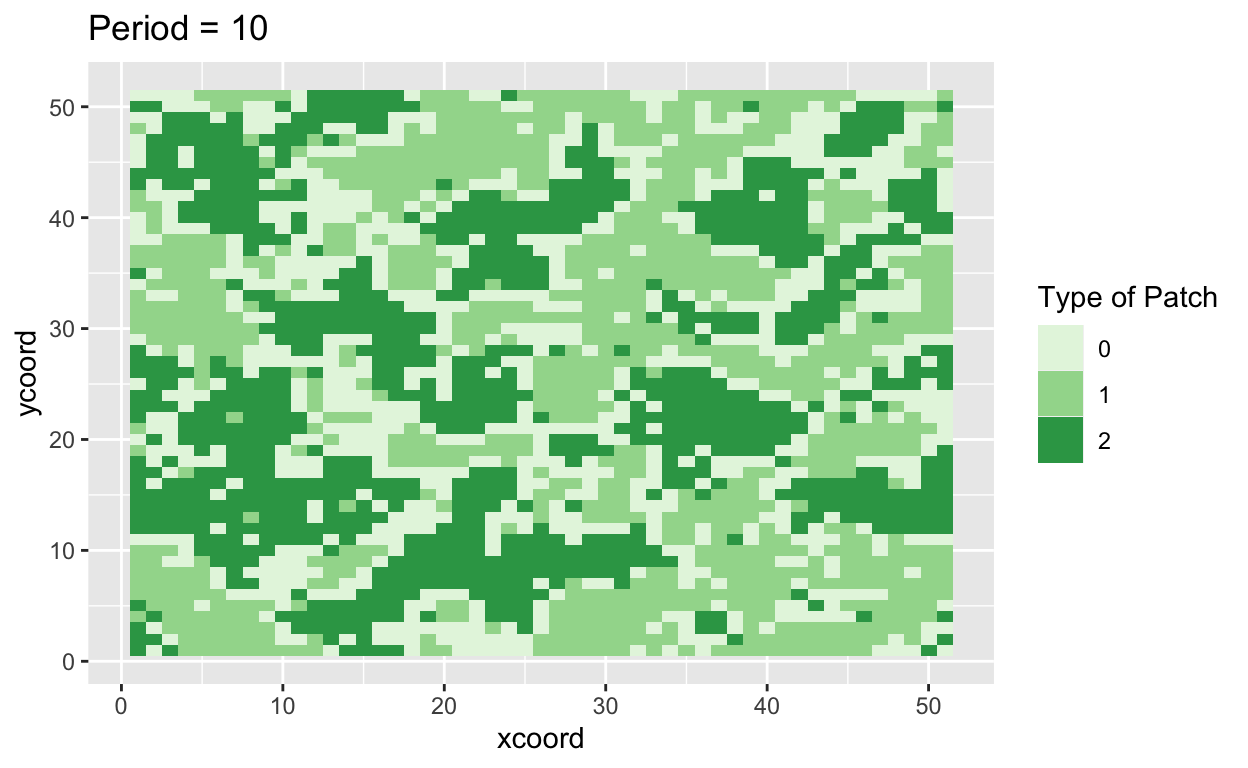
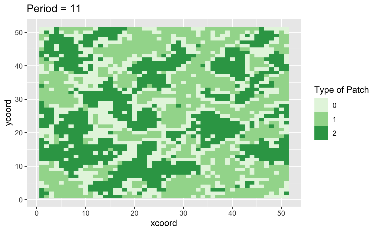
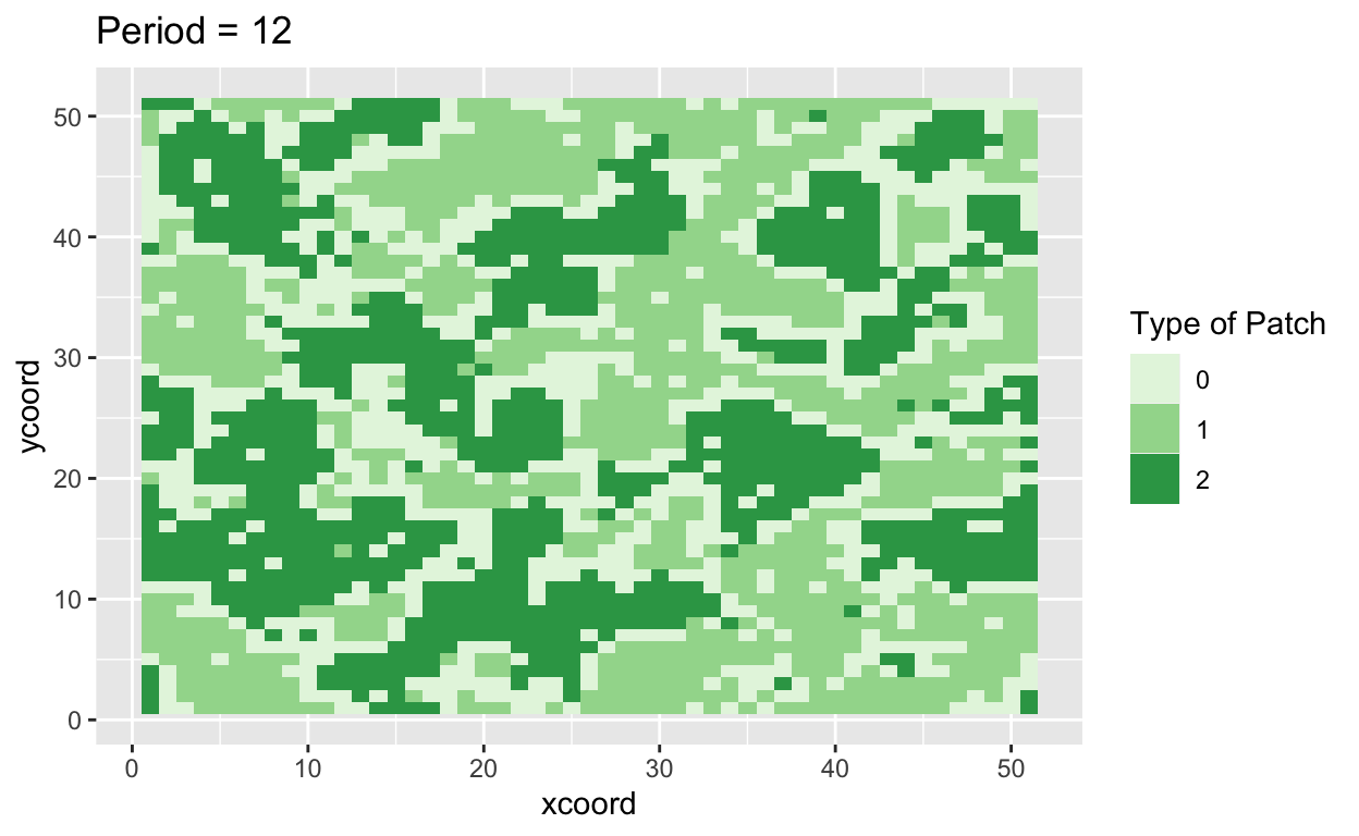
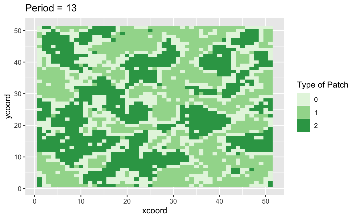
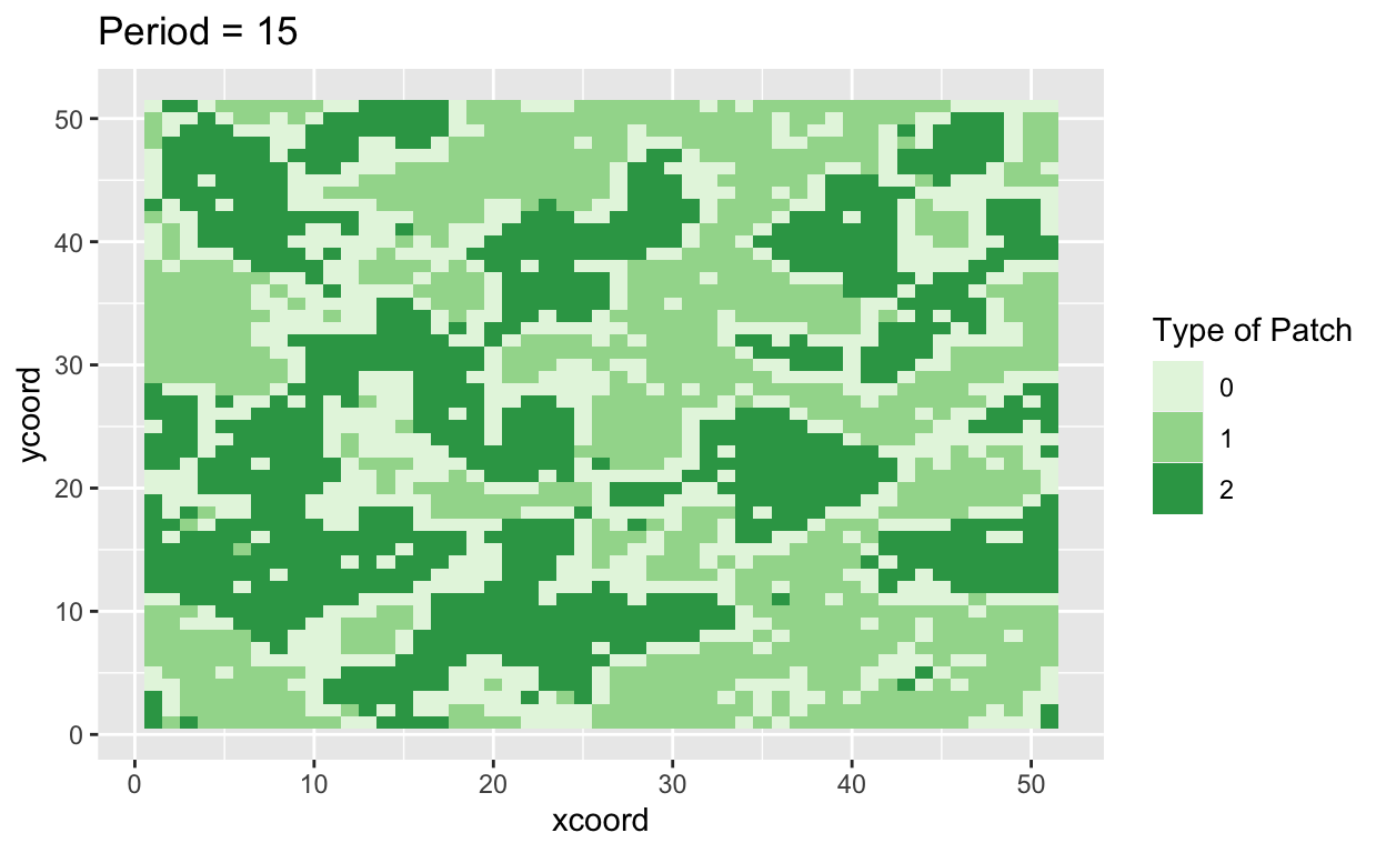
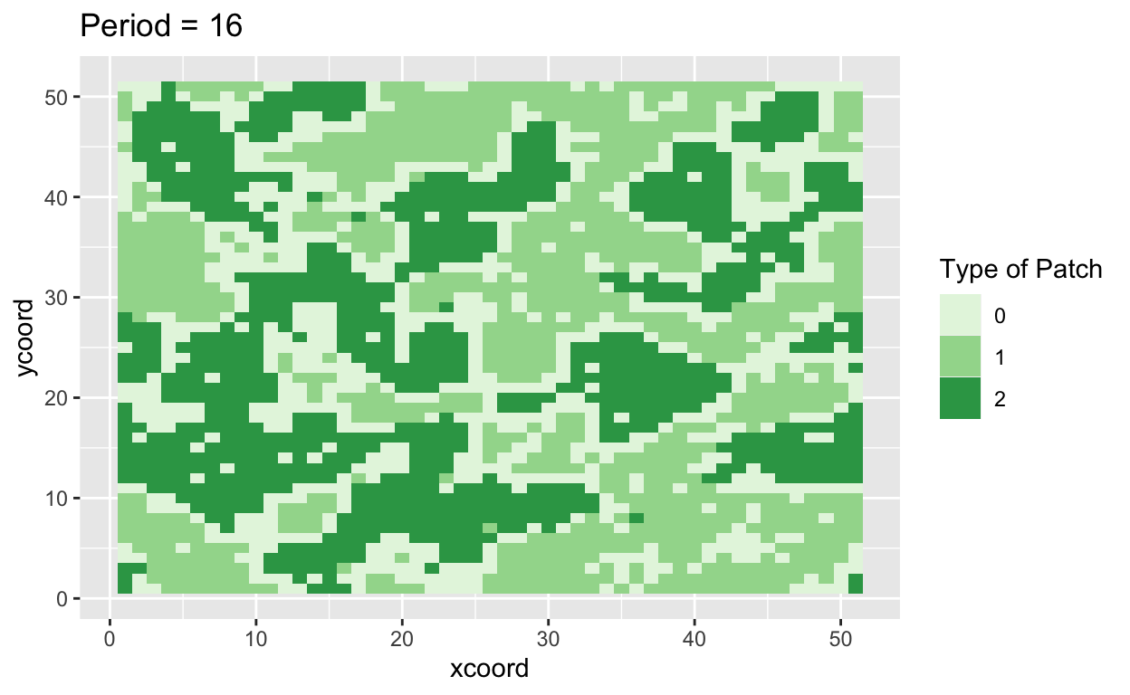
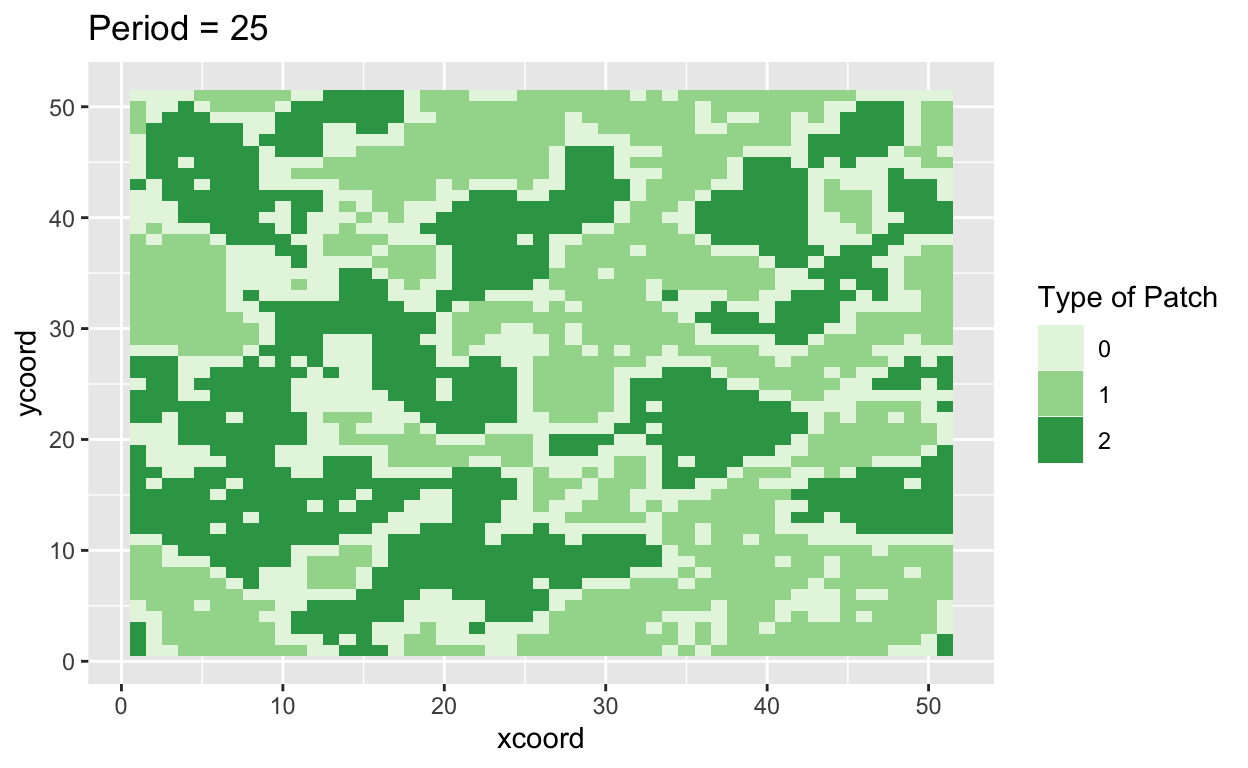
gp <- ggplot(patch_df, aes(x = xcoord, y = ycoord, fill = factor(type))) +
geom_tile() +
ggtitle(paste("Period =", i)) +
scale_fill_brewer(palette = "Greens",
name = "Type of Patch")
save_plots[[i]] <- gp
}
ggplot(plotfirst, aes(x = xcoord, y = ycoord, fill = factor(type))) +
  geom_tile() +
  ggtitle("Period = 0") +
  scale_fill_brewer(palette = "Greens",
                    name = "Type of Patch")
for(l in 1:time){

  print(save_plots[[l]])

}


ps, here is a ggplot tool for creating waffle plots.
Bo\(^2\)m =)