A replication of Thomas Schelling’s model, which was originally published in The Journal of Mathematical Sociology. Yuk Tung Liu offers a great summary.
The following map shows the distribution of people with different ethnicity living in the city of Chicago (source: radicalcartography.net):

Segregation may arise from social and economic reasons. However, Thomas Schelling, winner of the 2005 Nobel Memorial Prize in Economic Sciences, pointed out another possible reason. He constructed a simple model and used pennies and nickels on a graph paper to demonstrate that segregation can develop naturally even though each individual is tolerant towards another group. For example, if everyone requires at least half of his neighbors to be of the same color, the final outcome is a high degree of segregation. What Schelling demonstrated was that the “macrobehavior” in a society may not reflect the “micromotives” of its individual members.
Schelling’s model is an example of an agent-based model for simulating the actions and interactions of autonomous agents (both individual or collective entities such as organizations or groups) on the overall system. Agent-based models are useful in simulating complex systems. An interesting phenomenon that can occur in a complex system is emergence, in which a structure or pattern arises in the system from the bottom up. As you will see, segregation is a result of emergence in the system described by the Schelling model. Members of each group do not consciously choose to live in a certain area, but the collective behavior of the individuals gives rise to segregation.
Schelling Model
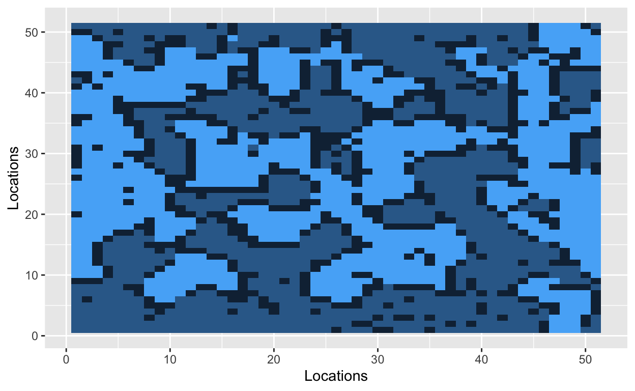
Let’s start by situating people on a grid. The cells of the grid will contain a value, and that value will indicate one of three states: uninhabited (0), inhabited by a hockey player (1), or inhabited by a soccer player (2). Let’s use a 51x51 grid with 2000 occupied cells. A 51x51 grid contains 2601 cells in total.
Create a vector with 1000s 1s, 1000 2s, and the remaining 601 slots 0s.
group
   0    1    2
 601 1000 1000
So far, all I have is a vector with a bunch of 1s, 2s, and 0s.
Now, collate those numbers into a matrix through random sampling.
[1] 2 2 2 1[1] 0 1 2 2 1[1] 1 0 0 0 1 0 0Plot with base R

Plot with ggplot2 - requires long data
  Var1 Var2 value
1    1    1     1
2    2    1     1
3    3    1     1
4    4    1     1
5    5    1     1
6    6    1     0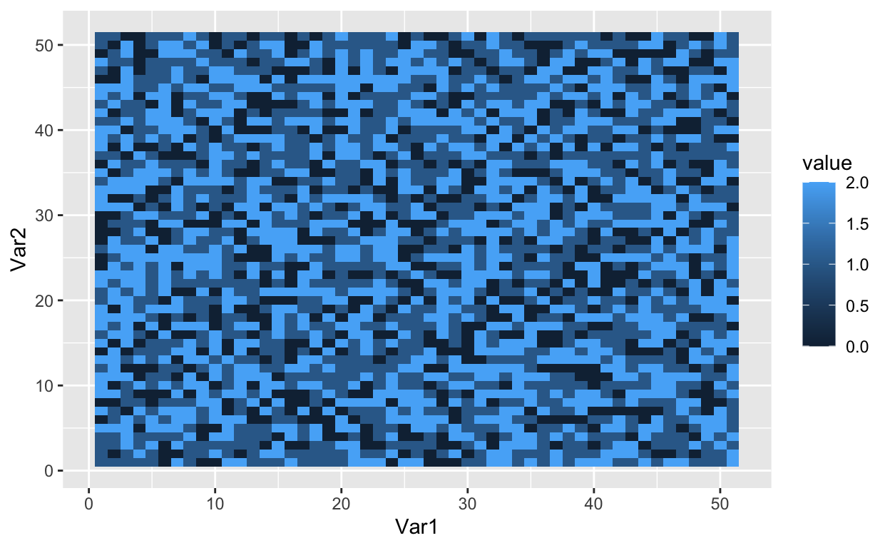
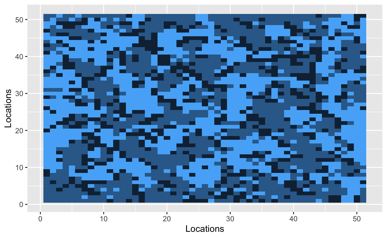
The grid is now filled with randomly dispersed hockey players, soccer players, and empty lots. The next step is to introduce a parameter that Schelling used in his original model. The similarity threshold, \(z\), takes a value between 0 and 1, and it measures how intolerant an agent is towards other athletes. An agent is satisfied if at least a fraction \(z\) of his neighbors belong to the same group – i.e., a hockey player likes to be around other hockey players. Mathematically, an agent is satisfied if the number of people around him is greater than \(z\). He is dissatisfied if he has fewer people of similar type around him. The smaller the value of \(z\), the more tolerant agents are of other groups.
With a similarity threshold of 0.30, a hockey player will move if fewer than 30% of his neighbors are other hockey players. A hockey player will stay if at least 30% of his neighbors are hockey players.
Having set the threshold, we now need a function to calculate how many neighbors are hockey players and how many are soccer players. This function spits back the similarity ratio, \(r_{sim}\). \(r_{sim}\) is a proportion: the number of neighbors of the same group divided by the total number of neighbors.
\[\begin{equation} r_{sim} = \dfrac{n_{same}}{n_{neighbors}} \end{equation}\]
For a hockey player, the ratio would become
\[\begin{equation} r_{sim_{hockey}} = \dfrac{n_{hockey}}{n_{neighbors}} \end{equation}\]
Here is an example:

If I were a super programmer, I could create a function to do so. I’m not. Instead, I’ll create a function called get_neighbor_coords that returns the locations of every neighbor for agent \(i\). The function takes a vector parameter that houses agent \(i\)s location (e.g., [2, 13]). Then, it pulls the coordinates of each neighbor under the Moore paradigm (8 surrounding patches - clockwise).
The function returns a matrix with the coordinates of the surrounding 8 patches. If I was focused, for example, on agent [2, 3], then the function would return
     [,1] [,2]
[1,]    3    3
[2,]    3    4
[3,]    2    4
[4,]    1    4
[5,]    1    3
[6,]    1    2
[7,]    2    2
[8,]    3    2
which shows that coordinate [3,3] is just below agent \(i\), coordinate [3,4] is just below and to the right, and coordinate [2,4] is directly to the right.
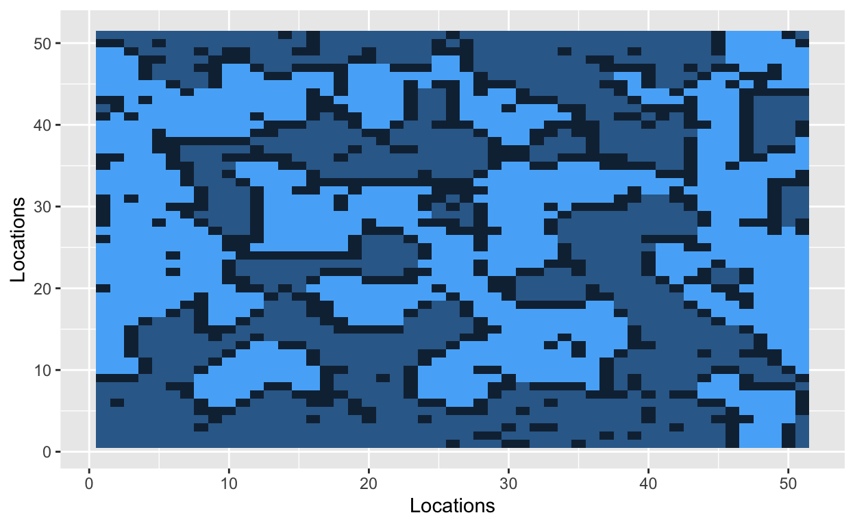
Now we are ready to iterate across every agent (i.e., every cell in grid).


Bo\(^2\)m =)