Think about what it would mean to explain something to a friend. How would you explain why the Patriot’s won the Superbowl? How would you explain why you are feeling happy or sad? How would you explain tying a shoe to a toddler? How would you explain why eating lots of donuts tends to increase a person’s weight? How would you explain the timeline of Game of Thrones to someone who hadn’t seen it?
What you came up with, or thought about, is different from how “explaining” is usually used in research. We typically use the term to mean “explain variation,” and the goal of this post is to flesh-out what that means. While you read this, though, try to keep in mind the thought, “how does this connect to the way I explain things in everyday life?”
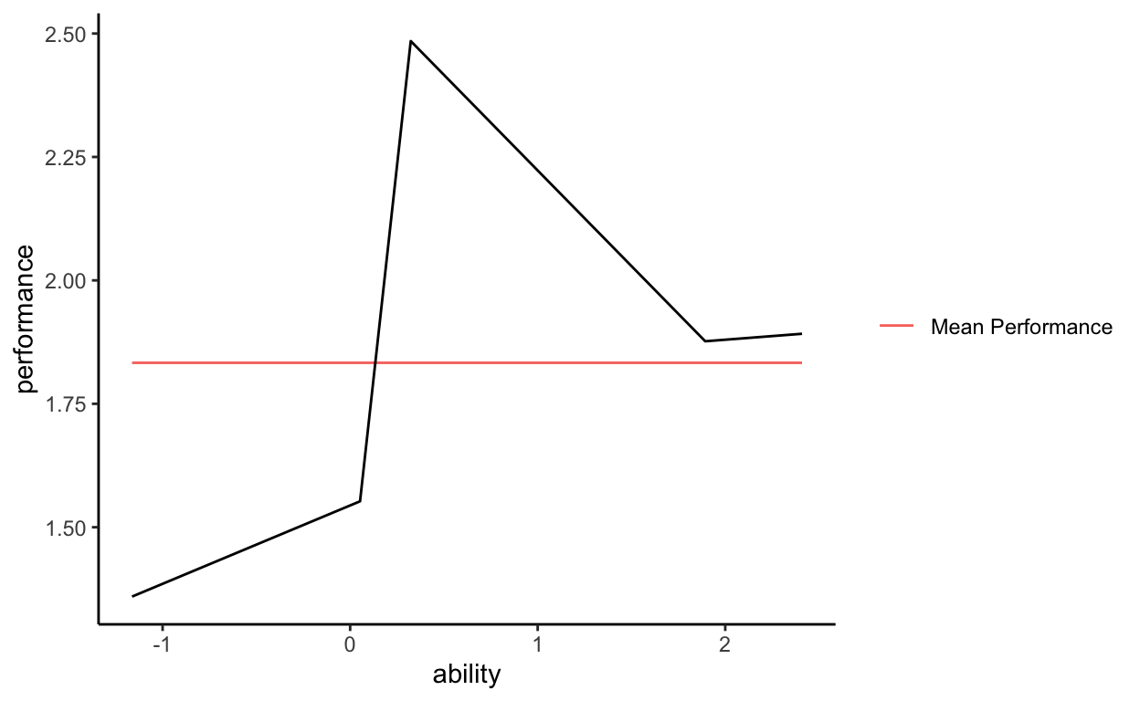
Imagine that we have a scatter plot, performance on the Y axis and ability on the X axis.
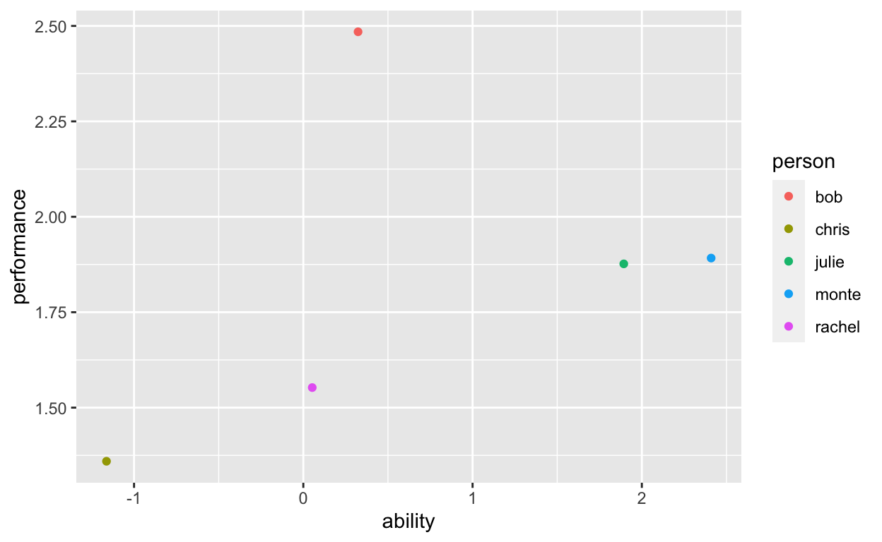
We collected data on several people – Bob, Chris, Julie, Monte, and Rachel, we measured each person’s performance and ability – and those individual data points are represented in the scatterplot. In statistics, what we try to do is account for variability in performance, we try to explain variation in performance. Here is what that means.
Take the mean of performance as a flat, horizontal line across all values of ability. For now we do not care about ability, we are just using it to visualize the data.
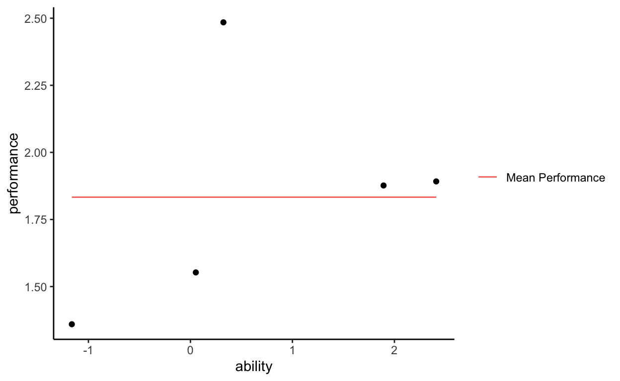
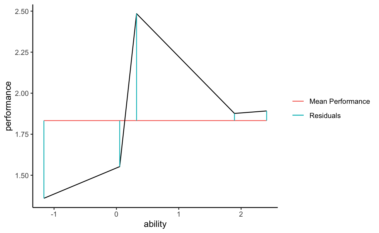
Notice that the mean of performance does not perfectly align with the observed data. That is, each of the points on the plot do not fall exactly on the horizontal line. If they did, we would say that the mean of performance perfectly explains the variability in performance. Instead, each of the points has some distance from the mean of performance line, and we call those distances residuals.
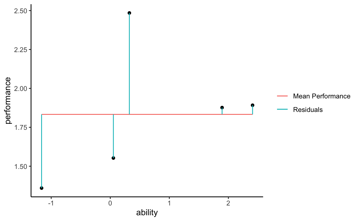
What those residuals mean conceptually is that the observed data points do not fall exactly on the mean of performance. Performance cannot be explained simply by its mean. There is variation in performance that is left to explain, there are distances (residuals) that are not accounted for.
Summing across all of those residuals gets us what is called the total sum of squares. All of the observed values have some distance from the mean performance line, when we aggregate all of those distances (all of the vertical line segments) we get an index of the variability in performance that we are trying to explain.
TSS = sum of vertical, residual distances
The real equation for TSS uses squares because negative distances will cancel positive distances, but this is a conceptual write-up. So we are ok ignoring that for now.
So, we have variation in performance that is not accounted for by the mean of performance. Now imagine that we believe some super complicated function of ability (X) explains the variation in performance. This super complicated function is a crazy line that perfectly runs through every observed data point.
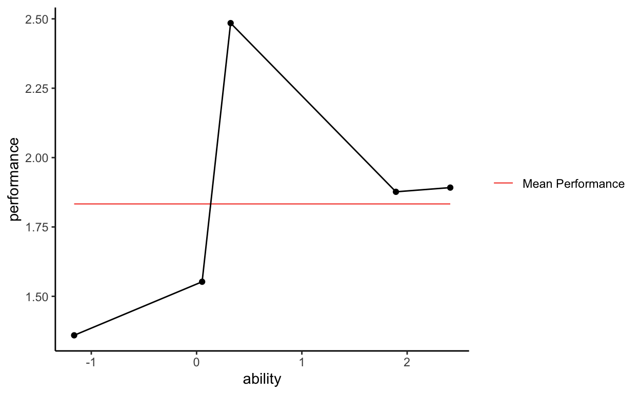
Now remove the observed data points from the graph so that we are only looking at the mean of performance and the predicted values of performance as a function of ability.
Now we have a graph of PREDICTED data. That is, the black line does not have observed data points, it does not represent what we saw when we collected data and measured performance and ability on Bob and the others. We are looking at the predicted values of performance based on some super complicated function of ability. Notice that the black line also has distances from the mean of performance, so we can sum across those distances to get another quantity, called the expected sum of squares.
ESS = sum of vertical, residual distances (but from our predicted line rather than our observed data points)
Because our super complicated function perfectly went through each observed data point, TSS is equivalent to ESS in this case. That means that our super complicated function perfectly explains the variation in performance. We have accounted for all variance in our outcome.
Usually we don’t use super complicated equations. We tend to posit linear functions, such that we think that performance is a linear function of ability. If we were to plot a predicted line showing performance as a linear function of ability, the residual distances would change and ESS would be different from TSS, meaning that we explained some, but not all of the variation in performance.
That is what explaining means in research and statistics (technically, “explaining variation”). Observed data varies about the mean on some dependent variable and there are distances from observed data points to the mean line. If we aggregate those distances together we get TSS, a sense of the total variation in the DV. Then we create some equation relating predictors to the outcome and use it to generate new values of the DV (i.e., predicted values). Explaining in statistics means, “to what extent do my predicted values have the same pattern of distances as my observed values?” “To what extent are the distances from the predicted values to the mean line the same as the distances from the observed values to the mean line?” “To what extent is the total variation represented by the predicted variation?” Is TSS equivalent to ESS?
Now return to the notion that we opened with, to what extent does explaining variation reflect how you explain things in everyday life?
Connecting to Causality
How does all of this connect to causality? Knowing about cause helps you “explain variation,” but explaining more or less variation does not give you information about cause. Said differently, knowledge about cause, or the data generating process, or truth, will influence your ability to explain variation, but improving your ability to explain variation will not necessarily produce insights about the DGP. If you know the true process – i.e., the DGP, the underlying structure of effects and variables, the causal system – then you will be able to (almost perfectly) explain variation in the sense that I described in this post. If you know the true process, then you will be able to explain why Bob’s score is different from Julie’s, why some variables correlate with the outcome and others don’t, and why Monte’s score is different from time 1 versus time 2. Full knowledge of the DGP means you can predict what happens next, there are no unknowns left to make your ESS different from your TSS.
But the reverse is not true. Just because you can explain variation – in the statistical sense described here – does not mean that you have the right DGP or know anything about cause. I could have the wrong DGP, the wrong notion about the causal structure, the wrong variables in the model, but improve my ability to “explain variation” by including more variables in my model. I could include additional, irrelevant variables to make my model more complex and subsequently improve my ability to “explain variation,” but I wouldn’t produce any greater knowledge about cause or the DGP. Knowledge about cause, explanation, why, or the DGP comes from research designs and assumptions, not statistical models. Did you randomly assign and manipulate, and were there strong assumptions involved in the form of DAGS? Did you “wiggle” or change some variables (think Judea Pearl) and observe the effect of doing so on other variables in a controlled environment? Fancy stats don’t get you there, great research designs and assumptions sometimes do.
Bo\(^2\)m =)