This post is about building intuition for degrees of freedom. There are two ways to think about it, the “information” way and the “line” way.
The Information Way
The quantity, degrees of freedom, is the amount of information available in our data set minus the amount of information we want to pull from it. Here are a bunch of different ways of representing that idea:
\[\begin{equation} \textrm{DF} = \textrm{Knowns} - \textrm{Unknowns} \end{equation}\]
\[\begin{equation} \textrm{DF} = \textrm{Unique information} - \textrm{Used information} \end{equation}\]
\[\begin{equation} \textrm{DF} = \textrm{Unique information in observed data} - \textrm{Information we want to pull from our data} \end{equation}\]
\[\begin{equation} \textrm{DF} = \textrm{Stuff in the correlation matrix} - \textrm{Stuff we want to use the correlation matrix for} \end{equation}\]
\[\begin{equation} \textrm{DF} = \textrm{Unique entries in the variance/covariance matrix} - \textrm{Estimated parameters} \end{equation}\]
In a data set, information is (roughly) the unique variances and covariances that I can use. If I estimate too many parameters without enough information (i.e., without enough observed variables), then I loose DFs and I can’t estimate anything. I cannot estimate a super complicated function if I only observe one measurement of performance and one measurement of motivation.
The Line Way
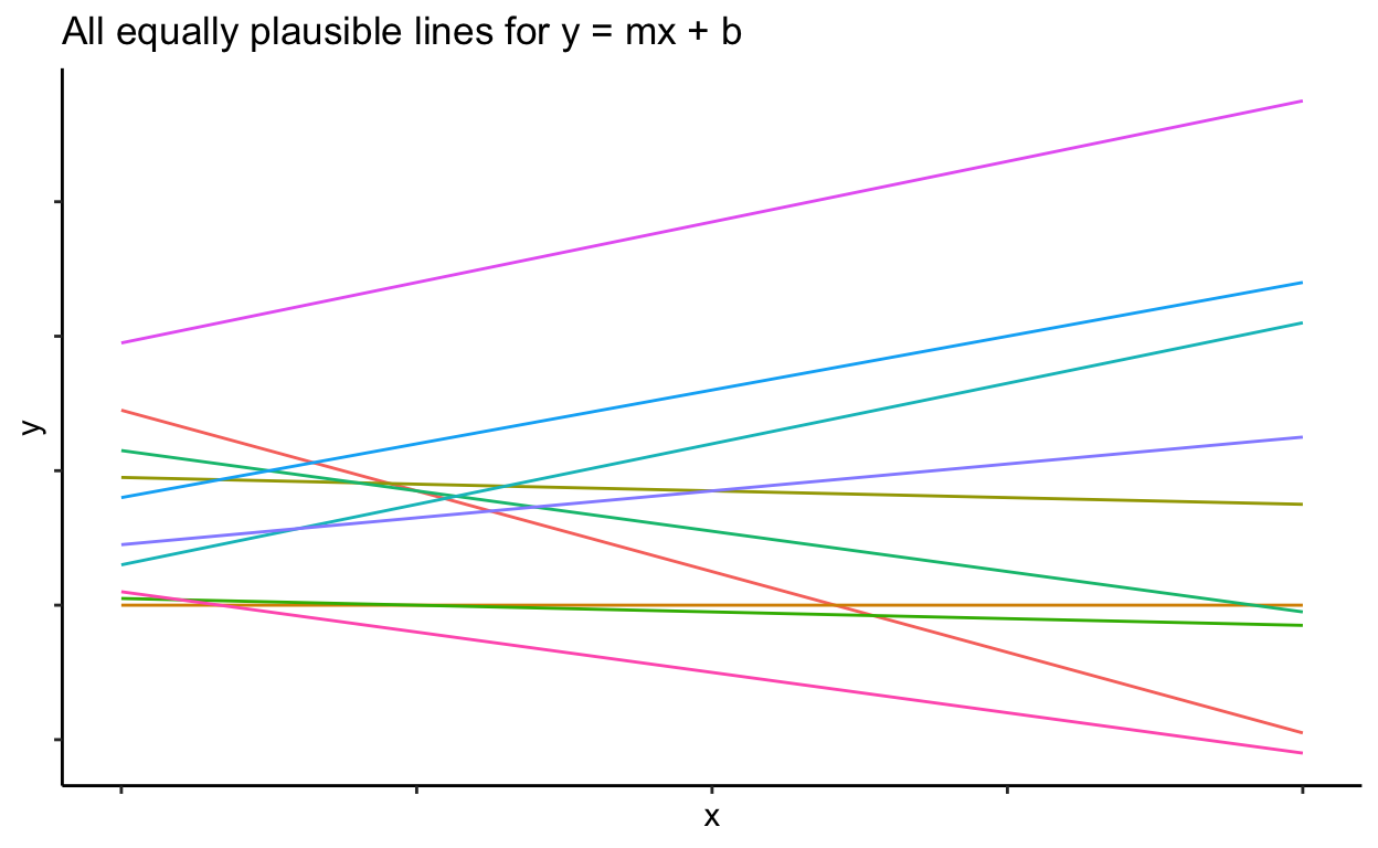
The line way builds off the idea that DF = unique information - used information, but we’re going to walk through it visually. Imagine the equation
\[\begin{equation} y = mx + b. \end{equation}\]
As written, an infinite number of lines can represent that equation. The intercept can be any value and the slope can be any value. There are no constraints.
Now imagine an equation with a constraint, such that the intercept must be 2:
\[\begin{equation} y = mx + 2. \end{equation}\]
You can still draw infinite lines here, but all of them must go through 2 as their intercept.

Now we can count our degrees of freedom. Let’s say each example above had 10 pieces of information (10 observed variables).
\[\begin{equation} y = mx + b \textrm{;} \textrm{ with 10 pieces of information and 2 estimated parameters. DF = 10 - 2. DF = 8} \end{equation}\]
\[\begin{equation} y = mx + 2 \textrm{;} \textrm{ with 10 pieces of information and 1 estimated parameter. DF = 10 - 1. DF = 9} \end{equation}\]
When you estimate an additional parameter you lose a degree of freedom. When you constrain things, you gain degrees of freedom. So, the second example has more degrees of freedom, even though it feels like we’re not as “free” to draw our lines. Tricky.
Bo\(^2\)m =)