Latent Growth Curves
I will progress through three models: linear, quadratic growth, and latent basis. In every example I use a sample of 400, 6 time points, and ‘affect’ as the variable of interest.
Don’t forget that multiplying by time
- \(0.6t\)
is different from describing over time
- \(0.6_t\).
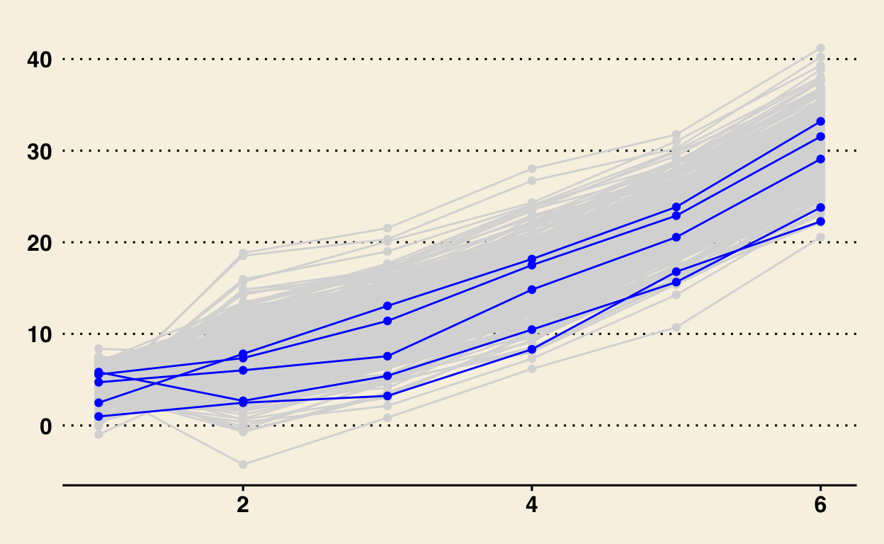
1) Linear
The data generating process:
\[\begin{equation} y_{it} = 4 - 0.6t + e_{t} \end{equation}\]
library(tidyverse)
library(ggplot2)
library(MASS)

N <- 400
time <- 6

intercept <- 4
linear_growth <- -0.6

df_matrix <- matrix(, nrow = N*time, ncol = 3)

count <- 0

for(i in 1:400){

  unob_het_affect <- rnorm(1,0,3)


  for(j in 1:6){

    count <- count + 1

    if(j == 1){

      df_matrix[count, 1] <- i
      df_matrix[count, 2] <- j
      df_matrix[count, 3] <- intercept + unob_het_affect + rnorm(1,0,1)
    }else{


      df_matrix[count, 1] <- i
      df_matrix[count, 2] <- j
      df_matrix[count, 3] <- intercept + linear_growth*j + unob_het_affect + rnorm(1,0,1)

    }


  }


}

df <- data.frame(df_matrix)
names(df) <- c('id', 'time', 'affect')

random_ids <- sample(df$id, 5)

random_df <- df %>%
  filter(id %in% random_ids)


ggplot(df, aes(x = time, y = affect, group = id)) +
  geom_point(color = 'gray85') +
  geom_line(color = 'gray85') +
  geom_point(data = random_df, aes(x = time, y = affect, group = id), color = 'blue') +
  geom_line(data = random_df, aes(x = time, y = affect, group = id), color = 'blue')

Estimating the model:
Formatting the data:
df_wide <- reshape(df, idvar = 'id', timevar = 'time', direction = 'wide')
First, an intercept only (no change) model:
library(lavaan)

no_change_string <- '

# Latent intercept factor

intercept_affect =~ 1*affect.1 + 1*affect.2 + 1*affect.3 + 1*affect.4 + 1*affect.5 + 1*affect.6

# Mean and variance of latent intercept factor

intercept_affect ~~ intercept_affect

# Fix observed variable means to 0

affect.1 ~ 0
affect.2 ~ 0
affect.3 ~ 0
affect.4 ~ 0
affect.5 ~ 0
affect.6 ~ 0

# Constrain residual (error) variance of observed variables to equality across time

affect.1 ~~ res_var*affect.1
affect.2 ~~ res_var*affect.2
affect.3 ~~ res_var*affect.3
affect.4 ~~ res_var*affect.4
affect.5 ~~ res_var*affect.5
affect.6 ~~ res_var*affect.6


'

no_change_model <- growth(no_change_string, data = df_wide)
summary(no_change_model, fit.measures = T)
lavaan 0.6-9 ended normally after 20 iterations

  Estimator                                         ML
  Optimization method                           NLMINB
  Number of model parameters                         8
  Number of equality constraints                     5

  Number of observations                           400

Model Test User Model:

  Test statistic                              2073.804
  Degrees of freedom                                24
  P-value (Chi-square)                           0.000

Model Test Baseline Model:

  Test statistic                              4042.863
  Degrees of freedom                                15
  P-value                                        0.000

User Model versus Baseline Model:

  Comparative Fit Index (CFI)                    0.491
  Tucker-Lewis Index (TLI)                       0.682

Loglikelihood and Information Criteria:

  Loglikelihood user model (H0)              -5203.688
  Loglikelihood unrestricted model (H1)      -4166.786

  Akaike (AIC)                               10413.376
  Bayesian (BIC)                             10425.350
  Sample-size adjusted Bayesian (BIC)        10415.831

Root Mean Square Error of Approximation:

  RMSEA                                          0.462
  90 Percent confidence interval - lower         0.445
  90 Percent confidence interval - upper         0.479
  P-value RMSEA <= 0.05                          0.000

Standardized Root Mean Square Residual:

  SRMR                                           0.194

Parameter Estimates:

  Standard errors                             Standard
  Information                                 Expected
  Information saturated (h1) model          Structured

Latent Variables:
                      Estimate  Std.Err  z-value  P(>|z|)
  intercept_affect =~
    affect.1             1.000
    affect.2             1.000
    affect.3             1.000
    affect.4             1.000
    affect.5             1.000
    affect.6             1.000

Intercepts:
                   Estimate  Std.Err  z-value  P(>|z|)
   .affect.1          0.000
   .affect.2          0.000
   .affect.3          0.000
   .affect.4          0.000
   .affect.5          0.000
   .affect.6          0.000
    intercept_ffct    2.067    0.153   13.509    0.000

Variances:
                   Estimate  Std.Err  z-value  P(>|z|)
    intrcp_           8.914    0.662   13.460    0.000
   .affct.1 (rs_v)    2.698    0.085   31.623    0.000
   .affct.2 (rs_v)    2.698    0.085   31.623    0.000
   .affct.3 (rs_v)    2.698    0.085   31.623    0.000
   .affct.4 (rs_v)    2.698    0.085   31.623    0.000
   .affct.5 (rs_v)    2.698    0.085   31.623    0.000
   .affct.6 (rs_v)    2.698    0.085   31.623    0.000
Now, a linear growth model centered at time point 1. The intercept factor estimate, therefore, is the estimated average affect at time 1.
library(lavaan)

linear_change_string <- '

# Latent intercept and slope factors

intercept_affect =~ 1*affect.1 + 1*affect.2 + 1*affect.3 + 1*affect.4 + 1*affect.5 + 1*affect.6
slope_affect =~ 0*affect.1 + 1*affect.2 + 2*affect.3 + 3*affect.4 + 4*affect.5 + 5*affect.6

# Mean and variance of latent factors

intercept_affect ~~ intercept_affect
slope_affect ~~ slope_affect

# Covariance between latent factors

intercept_affect ~~ slope_affect

# Fix observed variable means to 0

affect.1 ~ 0
affect.2 ~ 0
affect.3 ~ 0
affect.4 ~ 0
affect.5 ~ 0
affect.6 ~ 0

# Constrain residual (error) variance of observed variables to equality across time

affect.1 ~~ res_var*affect.1
affect.2 ~~ res_var*affect.2
affect.3 ~~ res_var*affect.3
affect.4 ~~ res_var*affect.4
affect.5 ~~ res_var*affect.5
affect.6 ~~ res_var*affect.6


'

linear_change_model <- growth(linear_change_string, data = df_wide)
summary(linear_change_model, fit.measures = T)
lavaan 0.6-9 ended normally after 48 iterations

  Estimator                                         ML
  Optimization method                           NLMINB
  Number of model parameters                        11
  Number of equality constraints                     5

  Number of observations                           400

Model Test User Model:

  Test statistic                                95.218
  Degrees of freedom                                21
  P-value (Chi-square)                           0.000

Model Test Baseline Model:

  Test statistic                              4042.863
  Degrees of freedom                                15
  P-value                                        0.000

User Model versus Baseline Model:

  Comparative Fit Index (CFI)                    0.982
  Tucker-Lewis Index (TLI)                       0.987

Loglikelihood and Information Criteria:

  Loglikelihood user model (H0)              -4214.395
  Loglikelihood unrestricted model (H1)      -4166.786

  Akaike (AIC)                                8440.790
  Bayesian (BIC)                              8464.738
  Sample-size adjusted Bayesian (BIC)         8445.700

Root Mean Square Error of Approximation:

  RMSEA                                          0.094
  90 Percent confidence interval - lower         0.075
  90 Percent confidence interval - upper         0.114
  P-value RMSEA <= 0.05                          0.000

Standardized Root Mean Square Residual:

  SRMR                                           0.034

Parameter Estimates:

  Standard errors                             Standard
  Information                                 Expected
  Information saturated (h1) model          Structured

Latent Variables:
                      Estimate  Std.Err  z-value  P(>|z|)
  intercept_affect =~
    affect.1             1.000
    affect.2             1.000
    affect.3             1.000
    affect.4             1.000
    affect.5             1.000
    affect.6             1.000
  slope_affect =~
    affect.1             0.000
    affect.2             1.000
    affect.3             2.000
    affect.4             3.000
    affect.5             4.000
    affect.6             5.000

Covariances:
                      Estimate  Std.Err  z-value  P(>|z|)
  intercept_affect ~~
    slope_affect         0.049    0.036    1.368    0.171

Intercepts:
                   Estimate  Std.Err  z-value  P(>|z|)
   .affect.1          0.000
   .affect.2          0.000
   .affect.3          0.000
   .affect.4          0.000
   .affect.5          0.000
   .affect.6          0.000
    intercept_ffct    3.806    0.154   24.653    0.000
    slope_affect     -0.696    0.011  -61.197    0.000

Variances:
                   Estimate  Std.Err  z-value  P(>|z|)
    intrcp_           8.992    0.674   13.336    0.000
    slp_ffc          -0.007    0.004   -1.712    0.087
   .affct.1 (rs_v)    1.030    0.036   28.284    0.000
   .affct.2 (rs_v)    1.030    0.036   28.284    0.000
   .affct.3 (rs_v)    1.030    0.036   28.284    0.000
   .affct.4 (rs_v)    1.030    0.036   28.284    0.000
   .affct.5 (rs_v)    1.030    0.036   28.284    0.000
.affct.6 (rs_v) 1.030 0.036 28.284 0.000inspect(linear_change_model, 'cov.lv')
                 intrc_ slp_ff
intercept_affect  8.992
slope_affect      0.049 -0.007
This model does an adequate job recovering the intercept and slope parameters.
If I wanted to center the model at time point 3 the latent intercept term would be interpreted as the estimated average affect at time 3 and the syntax would change to:
'
slope_affect =~ -2*affect.1 + -1*affect.2 + 0*affect.3 + 1*affect.4 + 2*affect.5 + 3*affect.6

'
2) Quadratic
The data generating process:
\[\begin{equation} y_{it} = 4 + 0.2t + 0.7t^2 + e_{t} \end{equation}\]
library(tidyverse)
library(ggplot2)
library(MASS)

N <- 400
time <- 6


intercept_mu <- 4
linear_growth2 <- 0.2
quad_growth <- 0.7

df_matrix2 <- matrix(, nrow = N*time, ncol = 3)

count <- 0

for(i in 1:400){

  unob_het_affect <- rnorm(1,0,3)


  for(j in 1:6){

    count <- count + 1

    if(j == 1){

      df_matrix2[count, 1] <- i
      df_matrix2[count, 2] <- j
      df_matrix2[count, 3] <- intercept + rnorm(1,0,1) + rnorm(1,0,1)
    }else{


      df_matrix2[count, 1] <- i
      df_matrix2[count, 2] <- j
      df_matrix2[count, 3] <- intercept + linear_growth2*j + quad_growth*(j^2) + unob_het_affect + rnorm(1,0,1)

    }


  }


}

df2 <- data.frame(df_matrix2)
names(df2) <- c('id', 'time', 'affect')

random_ids2 <- sample(df2$id, 5)

random_df2 <- df2 %>%
  filter(id %in% random_ids2)


ggplot(df2, aes(x = time, y = affect, group = id)) +
  geom_point(color = 'gray85') +
  geom_line(color = 'gray85') +
  geom_point(data = random_df2, aes(x = time, y = affect, group = id), color = 'blue') +
  geom_line(data = random_df2, aes(x = time, y = affect, group = id), color = 'blue') +
  theme_wsj()
Estimating the model:
Quadratic growth model:
df_wide2 <- reshape(df2, idvar = 'id', timevar = 'time', direction = 'wide')


library(lavaan)

quad_change_string <- [1012 chars quoted with ''']

quad_change_model <- growth(quad_change_string, data = df_wide2)
summary(quad_change_model, fit.measures = T)
lavaan 0.6-9 ended normally after 82 iterations

  Estimator                                         ML
  Optimization method                           NLMINB
  Number of model parameters                        15
  Number of equality constraints                     5

  Number of observations                           400

Model Test User Model:

  Test statistic                               609.350
  Degrees of freedom                                17
  P-value (Chi-square)                           0.000

Model Test Baseline Model:

  Test statistic                              3203.346
  Degrees of freedom                                15
  P-value                                        0.000

User Model versus Baseline Model:

  Comparative Fit Index (CFI)                    0.814
  Tucker-Lewis Index (TLI)                       0.836

Loglikelihood and Information Criteria:

  Loglikelihood user model (H0)              -4603.247
  Loglikelihood unrestricted model (H1)      -4298.572

  Akaike (AIC)                                9226.494
  Bayesian (BIC)                              9266.409
  Sample-size adjusted Bayesian (BIC)         9234.678

Root Mean Square Error of Approximation:

  RMSEA                                          0.295
  90 Percent confidence interval - lower         0.275
  90 Percent confidence interval - upper         0.315
  P-value RMSEA <= 0.05                          0.000

Standardized Root Mean Square Residual:

  SRMR                                           0.223

Parameter Estimates:

  Standard errors                             Standard
  Information                                 Expected
  Information saturated (h1) model          Structured

Latent Variables:
                       Estimate  Std.Err  z-value  P(>|z|)
  intercept_affect =~
    affect.1              1.000
    affect.2              1.000
    affect.3              1.000
    affect.4              1.000
    affect.5              1.000
    affect.6              1.000
  slope_affect =~
    affect.1              0.000
    affect.2              1.000
    affect.3              2.000
    affect.4              3.000
    affect.5              4.000
    affect.6              5.000
  quad_slope_affect =~
    affect.1              0.000
    affect.2              1.000
    affect.3              4.000
    affect.4              9.000
    affect.5             16.000
    affect.6             25.000

Covariances:
                      Estimate  Std.Err  z-value  P(>|z|)
  intercept_affect ~~
    slope_affect         0.897    0.148    6.066    0.000
    quad_slop_ffct      -0.136    0.024   -5.748    0.000
  slope_affect ~~
    quad_slop_ffct      -0.461    0.049   -9.468    0.000

Intercepts:
                   Estimate  Std.Err  z-value  P(>|z|)
   .affect.1          0.000
   .affect.2          0.000
   .affect.3          0.000
   .affect.4          0.000
   .affect.5          0.000
   .affect.6          0.000
    intercept_ffct    4.226    0.069   60.965    0.000
    slope_affect      2.163    0.103   20.974    0.000
    quad_slop_ffct    0.610    0.017   36.907    0.000

Variances:
                   Estimate  Std.Err  z-value  P(>|z|)
    intrcp_           0.626    0.146    4.288    0.000
    slp_ffc           3.107    0.304   10.205    0.000
    qd_slp_           0.067    0.008    8.463    0.000
   .affct.1 (rs_v)    1.579    0.064   24.495    0.000
   .affct.2 (rs_v)    1.579    0.064   24.495    0.000
   .affct.3 (rs_v)    1.579    0.064   24.495    0.000
   .affct.4 (rs_v)    1.579    0.064   24.495    0.000
   .affct.5 (rs_v)    1.579    0.064   24.495    0.000
   .affct.6 (rs_v)    1.579    0.064   24.495    0.000
This model recovers the intercept and quadratic parameters but not the linear growth parameter.
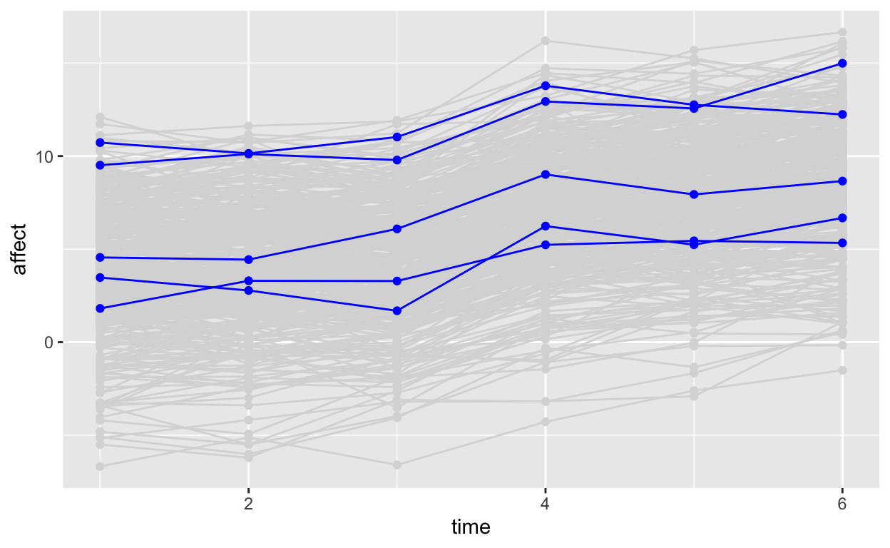
3) Latent Basis
This model allows us to see where a majority of the change occurs in the process. For example, does more change occur between time points 2 and 3 or 5 and 6? In this model we are not trying to recover the parameters, but describe the change process in detail.
Data generating process:
Time 1 - Time 3: \[\begin{equation} y_{it} = 4 + 0.2t + e_{t} \end{equation}\]
Time 4 - Time 6: \[\begin{equation} y_{it} = 4 + 0.8t + e_{t} \end{equation}\]
library(tidyverse)
library(ggplot2)
library(MASS)

N <- 400
time <- 6


intercept_mu <- 4
growth_1 <- 0.2
growth_2 <- 0.8


df_matrix3 <- matrix(, nrow = N*time, ncol = 3)

count <- 0

for(i in 1:400){

  unob_het_affect <- rnorm(1,0,3)


  for(j in 1:6){

    count <- count + 1

    if(j < 4){

      df_matrix3[count, 1] <- i
      df_matrix3[count, 2] <- j
      df_matrix3[count, 3] <- intercept + growth_1*j + unob_het_affect + rnorm(1,0,1)

    }else{


      df_matrix3[count, 1] <- i
      df_matrix3[count, 2] <- j
      df_matrix3[count, 3] <- intercept + growth_2*j + unob_het_affect + rnorm(1,0,1)

    }


  }


}

df3 <- data.frame(df_matrix3)
names(df3) <- c('id', 'time', 'affect')

random_ids3 <- sample(df3$id, 5)

random_df3 <- df3 %>%
  filter(id %in% random_ids3)


ggplot(df3, aes(x = time, y = affect, group = id)) +
  geom_point(color = 'gray85') +
  geom_line(color = 'gray85') +
  geom_point(data = random_df3, aes(x = time, y = affect, group = id), color = 'blue') +
  geom_line(data = random_df3, aes(x = time, y = affect, group = id), color = 'blue')
Estimating the model:
Latent basis:
Similar to a linear growth model but we freely estimate the intermediate basis coefficients. Remember to constrain the first basis coefficient to zero and the last to 1.
df_wide3 <- reshape(df3, idvar = 'id', timevar = 'time', direction = 'wide')


library(lavaan)

lb_string <- '

# Latent intercept and slope terms with intermediate time points freely estimated

intercept_affect =~ 1*affect.1 + 1*affect.2 + 1*affect.3 + 1*affect.4 + 1*affect.5 + 1*affect.6
slope_affect =~ 0*affect.1 + bc1*affect.2 + bc2*affect.3 + bc3*affect.4 + bc4*affect.5 + 1*affect.6

# Mean and variance of latent factors

intercept_affect ~~ intercept_affect
slope_affect ~~ slope_affect

# Covariance between latent factors

intercept_affect ~~ slope_affect

# Fix observed variable means to 0

affect.1 ~ 0
affect.2 ~ 0
affect.3 ~ 0
affect.4 ~ 0
affect.5 ~ 0
affect.6 ~ 0

# Constrain residual (error) variance of observed variables to equality across time

affect.1 ~~ res_var*affect.1
affect.2 ~~ res_var*affect.2
affect.3 ~~ res_var*affect.3
affect.4 ~~ res_var*affect.4
affect.5 ~~ res_var*affect.5
affect.6 ~~ res_var*affect.6


'

lb_model <- growth(lb_string, data = df_wide3)
summary(lb_model, fit.measures = T)
lavaan 0.6-9 ended normally after 64 iterations

  Estimator                                         ML
  Optimization method                           NLMINB
  Number of model parameters                        15
  Number of equality constraints                     5

  Number of observations                           400

Model Test User Model:

  Test statistic                                17.043
  Degrees of freedom                                17
  P-value (Chi-square)                           0.451

Model Test Baseline Model:

  Test statistic                              4190.601
  Degrees of freedom                                15
  P-value                                        0.000

User Model versus Baseline Model:

  Comparative Fit Index (CFI)                    1.000
  Tucker-Lewis Index (TLI)                       1.000

Loglikelihood and Information Criteria:

  Loglikelihood user model (H0)              -4202.053
  Loglikelihood unrestricted model (H1)      -4193.532

  Akaike (AIC)                                8424.107
  Bayesian (BIC)                              8464.021
  Sample-size adjusted Bayesian (BIC)         8432.291

Root Mean Square Error of Approximation:

  RMSEA                                          0.003
  90 Percent confidence interval - lower         0.000
  90 Percent confidence interval - upper         0.045
  P-value RMSEA <= 0.05                          0.973

Standardized Root Mean Square Residual:

  SRMR                                           0.018

Parameter Estimates:

  Standard errors                             Standard
  Information                                 Expected
  Information saturated (h1) model          Structured

Latent Variables:
                      Estimate  Std.Err  z-value  P(>|z|)
  intercept_affect =~
    affect.1             1.000
    affect.2             1.000
    affect.3             1.000
    affect.4             1.000
    affect.5             1.000
    affect.6             1.000
  slope_affect =~
    affect.1             0.000
    affect.2 (bc1)       0.056    0.015    3.799    0.000
    affect.3 (bc2)       0.095    0.015    6.550    0.000
    affect.4 (bc3)       0.666    0.013   49.749    0.000
    affect.5 (bc4)       0.827    0.014   58.819    0.000
    affect.6             1.000

Covariances:
                      Estimate  Std.Err  z-value  P(>|z|)
  intercept_affect ~~
    slope_affect        -0.086    0.158   -0.546    0.585

Intercepts:
                   Estimate  Std.Err  z-value  P(>|z|)
   .affect.1          0.000
   .affect.2          0.000
   .affect.3          0.000
   .affect.4          0.000
   .affect.5          0.000
   .affect.6          0.000
    intercept_ffct    3.921    0.167   23.461    0.000
    slope_affect      4.647    0.069   67.762    0.000

Variances:
                   Estimate  Std.Err  z-value  P(>|z|)
    intrcp_          10.178    0.746   13.651    0.000
    slp_ffc          -0.111    0.074   -1.499    0.134
   .affct.1 (rs_v)    0.996    0.035   28.284    0.000
   .affct.2 (rs_v)    0.996    0.035   28.284    0.000
   .affct.3 (rs_v)    0.996    0.035   28.284    0.000
   .affct.4 (rs_v)    0.996    0.035   28.284    0.000
   .affct.5 (rs_v)    0.996    0.035   28.284    0.000
   .affct.6 (rs_v)    0.996    0.035   28.284    0.000
bc1 represents the percentage of change for the average individual between time 1 and 2. bc2 represents the percentage change betwen time 1 and 3, bc4 is the percentage change between time 1 and 5, etc.
Bo\(^2\)m =)