Integration

Trapezoid Rule

To find the area under a curve we can generate a sequence of trapezoids that follow the rules of the curve (i.e., the data generating function for the curve) along the \(x\)-axis and then add all of the trapezoids together. To create a trapezoid we use the following equation:

let \(w\) equal the width of the trapezoid (along the \(x\)-axis), then
- Area = (\(w/2\) * \(f(x_i)\)) + \(f(x_i+1)\)

for a single trapezoid. That procedure then iterates across our entire \(x\)-axis and adds all of the components together.

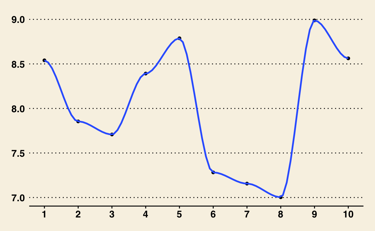
Here is an example function: \(f(x) = 8 + cos(x^3)\) and we will evaluate it over the interval [1, 10]. First, a plot of the curve itself.

x <- seq(from = 1, to = 10, by = 1)

f_x <- 8 + cos(x^3)



# Plot

library(ggplot2)
library(ggthemes)

ex_plot <- data.frame(
  "x" = c(x),
  "y" = c(f_x)
)

g_plot <- ggplot(ex_plot, aes(x = x, y = y)) + 
  geom_point() + 
  geom_smooth(se = F, span = 0.2) + 
  scale_x_continuous(breaks = c(1:10)) + 
  theme_wsj()

g_plot

The trapezoid algorithm:

# Parameters = the function, x-axis beginning, x-axis end, the number of trapezoids to create

trapezoid_rule <- function(fx, start, end, num_traps){
  
  # The width of each trapezoid
  
  w <- (end - start) / num_traps
  
  # the x-axis to evaluate our function along
  
  x_axis <- seq(from = start, to = end, by = w)
  
  # the y axis: apply the function (fx) to each value of our x-axis
  
  y_axis <- sapply(x_axis, fx)
  
  # The trapezoid rule: find the area of each trapezoid and then add them together
  
  trap_total <- w * ( (y_axis[1] / 2) + sum(y_axis[2:num_traps]) + (y_axis[num_traps + 1] / 2) )
  
  return(trap_total)
  
}

Now we can evaluate our function (\(f(x) = 8 + cos(x^3)\)) with our trapezoid algorithm to find the area under its curve.

Using only 3 trapezoids:

eval_function <- function(x){
  
  8 + cos(x^3)
  
}

trapezoid_rule(eval_function, 1, 10, 3)

[1] 72.29808

Using 10 trapezoids:

trapezoid_rule(eval_function, 1, 10, 10)

[1] 72.84693

Using 50000 trapezoids:

trapezoid_rule(eval_function, 1, 10, 50000)

[1] 71.84439

Optimization

The Golden-Section Method

Newton’s methods are great for finding local maxima or minima, but they also require knowing the derivative of whatever function we are evaluating. The goldent section method does not, and works in the following way:

Define three points along the x-axis: left (\(l\)), right (\(r\)), and middle (\(m\))
Choose one of the following sections along the \(x\)-axis according to which is larger:
- middle to right (section “right”)
- middle to left (section “left”)
Choose a point on the \(x\)-axis within section “right” according to the ‘golden rule’ (for our purposes the specifics of the golden rule are not important)
- Apply our function to \(y\) and \(m\)
  - If \(f(y)\) > \(f(m)\), then \(l\) becomes \(m\) and \(m\) becomes \(y\)
  - Else \(r\) becomes \(y\)
Choose a point on the \(x\)-axis within section “left” according to the ‘golden rule’ (for our purposes the specifics of the golden rule are not important)
- Apply our function to \(y\) and \(m\)
  - If \(f(y)\) > \(f(m)\), then \(r\) becomes \(m\) and \(m\) becomes \(y\)
  - Else \(l\) becomes \(y\)
Continue until the size of the “right” or “left” window diminishes to some a priori set tolerance value

Note that this method assumes that the

Now in code:

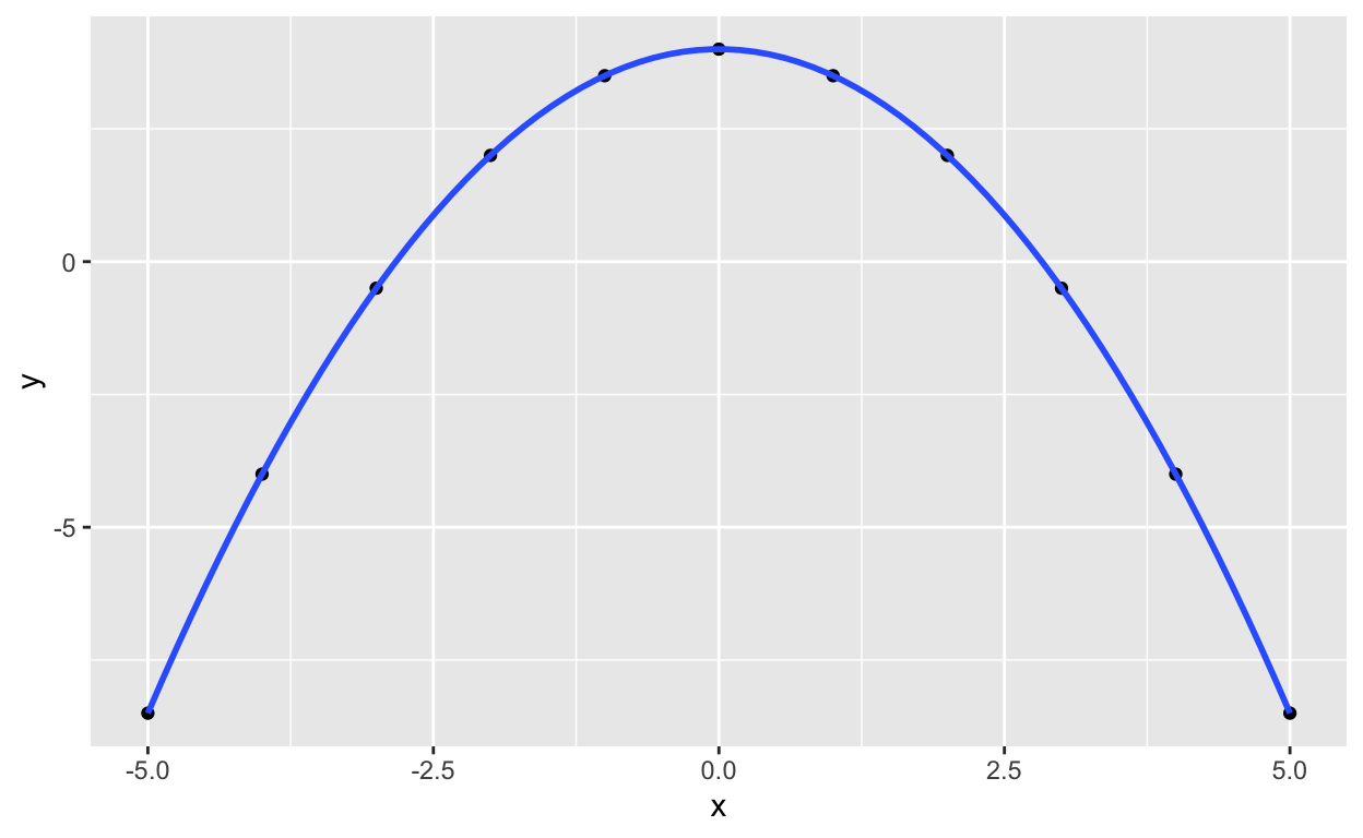
Our example function: \(f(x) = sin(x * 3)\)

x_2 <- seq(from = -5, to = 5, by = 1)

f_x_2 <- -0.5 * (x_2^2) + 4


# Plot

library(ggplot2)

ex_plot_2 <- data.frame(
  "x" = c(x_2),
  "y" = c(f_x_2)
)

g_plot_2 <- ggplot(ex_plot_2, aes(x = x, y = y)) + 
  geom_point() + 
  geom_smooth(se = F)

g_plot_2

The golden section algorithm:

golden_section <- function(fx, x.l, x.r, x.m, tolerance){
  
  # The golden ratio rule to help select 'y' when needed
  
  grule <- 1 + (1 * sqrt(5)) / 2
  
  # Apply the function at each of our starting locations (left, right, middle)
  
  # left
  
  f.l <- fx(x.l)
  
  # right
  
  f.r <- fx(x.r)
  
  # middle
  
  f.m <- fx(x.m)
  
  # continue to iterate until we pass our tolderance level for how big the "right" "left" window should be
  
  while (( x.r - x.l) > tolerance){
    
    
    # if the right window is larger than the left window, then operate on the right window side
    
    if ( (x.r - x.m) > (x.m - x.l) ){
      
      # select a point, y, according to the golden ratio rule
      
      y <- x.m + (x.r - x.m) / grule
      
      # apply the function to our selected y point
      
      f.y <- fx(y)
      
      # if the function at point y is higher than the function at the mid point
      
      if(f.y >= f.m){
        
        # reassign our points according to the algorithm steps outlined above
        
        # in this case, within the right window y was higher than the middle. So 'left' needs to become our new middle, and 'middle' needs to become y
        
        x.l <- x.m
        f.l <- f.m
        
        x.m <- y
        f.m <- f.y
      } else {
        
        # if the function at y was lower than the function at the mid point
        
        # shift 'right' to our y point
        
        x.r <- y
        f.r <- f.y
        
      }
      
      
      
      
      
    } else{
      
      # if the right window is not larger than the left window, select the left window to operate on
      
      
      # choose a point, y, within the left window according to the golden ratio
      
      y <- x.m - (x.m - x.l) / grule
      
      # apply our function to that point
      
      f.y <- fx(y)
      
      
      # if the function at y is greater than the function at the mid point (within the left window)
      
      if(f.y >= f.m){
        
        # reassign values according to the golden section method discussed above
        
        # in this case, within the left window our selected point is higher than the mid point (which is to the right of the selected y point)
        # so our "mid" point needs to become our "right" point and y needs to become "left"
        
        x.r <- x.m
        f.r <- f.m
        
        x.m <- y
        f.m <- f.y
        
        
        
      }else{
        
        # if the y point is lower than the function at the mid point
        
        # now our y needs to become "left"
        
        x.l <- y
        f.l <- f.y
      }
      
      
    }
    
    
    
  }
  
  # return the mid point
  
  return(x.m)
  
}

To summarize, the algorithm splits the \(x\)-axis into windows (left, middle, right) and then evaluates the function across those windows. The dimensions of the windows change over time depending on whether the function at \(y\) is higher or lower than a specific window dimension.

These examples are described in more detail in Jones, Maillardet, and Robinson, Introduction to Scientific Programming and Simulation Using R

Bo\(^2\)m =)

Numerical Integration and Optimization

Integration

Optimization