Random Walks

Some random walk fun. I use 400 steps in each example.

One-Dimensional Random Walk

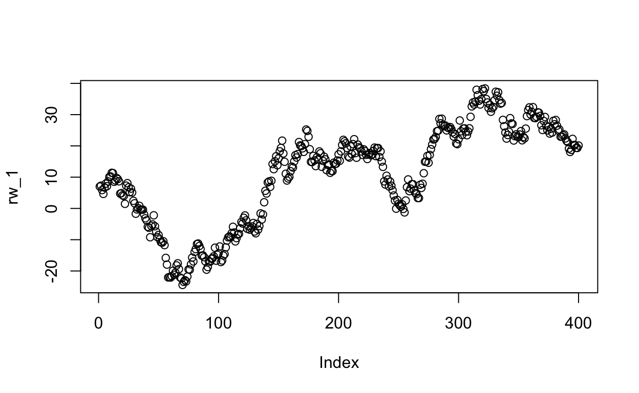
A random walk using a recursive equation.

# Empty vector to store the walk

rw_1 <- numeric(400)

# Initial value

rw_1[1] <- 7

# The Random Walk equation in a for-loop

for(i in 2:400){
  
  rw_1[i] <- 1*rw_1[i - 1] + rnorm(1,0,2)
  
}

plot(rw_1)

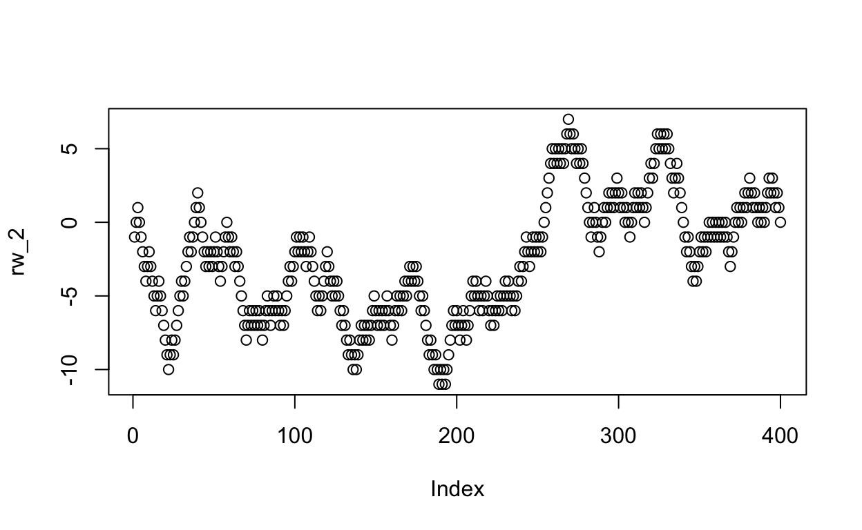
A random walk using R’s “cumsum” command. Here, I will generate a vector of randomly selected 1’s and -1’s. “Cumsum” then compiles those values.

# A vector of 1's and -1's

rw_2 <- sample(c(1, -1), 400, replace = T)

rw_2 <- cumsum(rw_2)

plot(rw_2)

Two-Dimensional Random Walk

Now for the real fun. Here, the walk can move forward (1) or backward (-1) along either dimension 1 or 2. So, if the walk moves forward (1) in dimension 1, dimension 2 receives a value of 0 for that step. If the walk moves backward (-1) in dimension 2, dimension 1 receives a 0 for that step.

# A matrix to store our walk

# Column 1 is dimension 1, column 2 is dimension 2

rw_3 <- matrix(0, ncol = 2, nrow = 400)

index <- cbind(
      1:400, sample(c(1, 2),
      400,
      replace = T)
)

The “index” merits some explaining. The walk will randomly choose to move in dimension 1 (column 1 in “rw_3”) or 2 (column 2 in “rw_3”). This index establishes a way of assigning which choice the walk makes. Here is what “index” looks like:

head(index)

     [,1] [,2]
[1,]    1    1
[2,]    2    1
[3,]    3    1
[4,]    4    2
[5,]    5    1
[6,]    6    1

The first column values tell the random walk which step its on (i.e., which row in “rw_3”), and the second column values tell the random walk which dimension it will step through (i.e., which column in “rw_3”).

So the “index” represents a random selection of dimension 1 or 2 at each step. Now I can apply that random choice to the random choice of stepping forward or backward (1 or -1).

# At each step, select a dimension (specified by the index; column 1 or 2 of rw_3)

# Then randomly select forward or backward

rw_3[index] <- sample(c(-1, 1), 
                      400, 
                      replace = T)



# Now sum each column (dimension) just like our 1-dimensional walks

rw_3[,1] <- cumsum(rw_3[,1])
rw_3[,2] <- cumsum(rw_3[,2])

Here is a visualization of the walk:

library(plotly)

rw_3 <- data.frame(rw_3)
rw_3$step <- c(1:400)

names(rw_3)[1:2] <- c("Dim_1", "Dim_2")

plot_ly(rw_3, x = ~step, y = ~Dim_1, z = ~Dim_2, type = 'scatter3d', mode = 'lines',
        line = list(color = '#1f77b4', width = 1))

Bo\(^2\)m =)